Linear regression is a great initial approach to take to model building. In fact, in the realm of statistical models, linear regression (calculated by ordinary least squares) is the best linear unbiased estimator. The two key pieces to that previous statement are “best” and “unbiased.”
What does it mean to be unbiased? Each of the sample coefficients (\(\hat{\beta}\)’s) in the regression model are estimates of the true coefficients. These sample coefficients have sampling distributions - specifically, normally distributed sampling distributions. The mean of the sampling distribution of \(\hat{\beta}_j\) is the true (unknown) coefficient \(\beta_j\). This means the coefficient is unbiased.
What does it mean to be best? IF the assumptions of ordinary least squares are met fully, then the sampling distributions of the coefficients in the model have the minimum variance of all unbiased estimators.
These two things combined seem like what we want in a model - estimating what we want (unbiased) and doing it in a way that has the minimum amount of variation (best among the unbiased). Again, these rely on the assumptions of linear regression holding true. Another approach to regression would be to use regularized regression instead as a different approach to building the model.
As the number of variables in a linear regression model increase, the chances of having a model that meets all of the assumptions starts to diminish. Multicollinearity can also pose a large problem with bigger regression models. The coefficients of a linear regression vary widely in the presence of multicollinearity. These variations lead to over-fitting of a regression model. More formally, these models have higher variance than desired. In those scenarios, moving out of the realm of unbiased estimates may provide a lower variance in the model, even though the model is no longer unbiased as described above. We wouldn’t want to be too biased, but some small degree of bias might improve the model’s fit overall and even lead to better predictions at the cost of a lack of interpretability.
Another potential problem for linear regression is when we have more variables than observations in our data set. This is a common problem in the space of genetic modeling. In this scenario, the ordinary least squares approach leads to multiple solutions instead of just one. Unfortunately, most of these infinite solutions over-fit the problem at hand anyway.
Regularized (or penalized or shrinkage) regression techniques potentially alleviate these problems. Regularized regression puts constraints on the estimated coefficients in our model and shrink these estimates to zero. This helps reduce the variation in the coefficients (improving the variance of the model), but at the cost of biasing the coefficients. The specific constraints that are put on the regression inform the three common approaches - ridge regression, LASSO, and elastic nets.
Penalties in Models
In ordinary least squares linear regression, we minimize the sum of the squared residuals (or errors).
As mentioned above, the penalties we choose constrain the estimated coefficients in our model and shrink these estimates to zero. Different penalties have different effects on the estimated coefficients. Two common approaches to adding penalties are the ridge and LASSO approaches. The elastic net approach is a combination of these two. Let’s explore each of these in further detail.
Ridge Regression
Ridge regression adds what is commonly referred to as an “\(L_2\)” penalty:
This penalty is controlled by the tuning parameter\(\lambda\). If \(\lambda = 0\), then we have typical OLS linear regression. However, as \(\lambda \rightarrow \infty\), the coefficients in the model shrink to zero. This makes intuitive sense. Since the estimated coefficients, \(\hat{\beta}_j\)’s, are the only thing changing to minimize this equation, then as \(\lambda \rightarrow \infty\), the equation is best minimized by forcing the coefficients to be smaller and smaller. We will see how to optimize this penalty term later in this section.
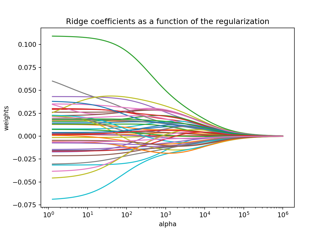
Here is a visual of the impact of adding more bias on the coefficients from our Ames housing model using a ridge regression:
Ridge(alpha=np.float64(1000000.0))
In a Jupyter environment, please rerun this cell to show the HTML representation or trust the notebook. On GitHub, the HTML representation is unable to render, please try loading this page with nbviewer.org.
Notice in the above plot that as the bias (represented by the x-axis) gets larger, the coefficients get closer to 0. However, those coefficients are asymptotically approaching 0 while never equaling it. This is different than the next approach!
LASSO
Least absolute shrinkage and selection operator (LASSO) regression adds what is commonly referred to as an “\(L_1\)” penalty:
This penalty is controlled by the tuning parameter\(\lambda\). If \(\lambda = 0\), then we have typical OLS linear regression. However, as \(\lambda \rightarrow \infty\), the coefficients in the model shrink to zero. This makes intuitive sense. Since the estimated coefficients, \(\hat{\beta}_j\)’s, are the only thing changing to minimize this equation, then as \(\lambda \rightarrow \infty\), the equation is best minimized by forcing the coefficients to be smaller and smaller. We will see how to optimize this penalty term later in this section.
However, unlike ridge regression that has the coefficient estimates approach zero asymptotically, in LASSO regression the coefficients can actually equal zero. This may not be as intuitive when initially looking at the penalty terms themselves. It becomes easier to see when dealing with the solutions to the coefficient estimates. Without going into too much mathematical detail, this is done by taking the derivative of the minimization function (objective function) and setting it equal to zero. From there we can determine the optimal solution for the estimated coefficients. In OLS regression the estimates for the coefficients can be shown to equal the following (in matrix form):
\[
\hat{\beta} = (X^TX)^{-1}X^TY
\]
This changes in the presence of penalty terms. For ridge regression, the solution becomes the following:
\[
\hat{\beta} = (X^TX + \lambda I)^{-1}X^TY
\]
There is no value for \(\lambda\) that can force the coefficients to be zero by itself. Therefore, unless the data makes the coefficient zero, the penalty term can only force the estimated coefficient to zero asymptotically as \(\lambda \rightarrow \infty\).
However, for LASSO, the solution isn’t quite as easy to show. However, in this scenario, there is a possible penalty value that will force the estimated coefficients to equal zero. There is some benefit to this. This makes LASSO also function as a variable selection criteria as well.
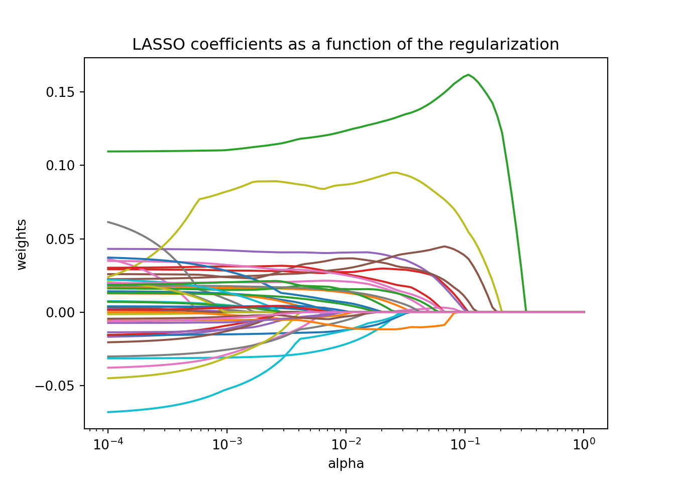
Here is a visual of the impact of adding more bias on the coefficients from our Ames housing model using a LASSO regression:
Lasso(alpha=np.float64(1.0), max_iter=5000)
In a Jupyter environment, please rerun this cell to show the HTML representation or trust the notebook. On GitHub, the HTML representation is unable to render, please try loading this page with nbviewer.org.
Notice in the above plot that as the bias (represented by the x-axis) gets larger, the coefficients get closer to 0. However, unlike ridge regression, there comes a point where a coefficient effectively gets zeroed out. Once that coefficient gets zeroed out, the model no longer is impacted by that variable which essentially removes the variable from the model.
Elastic Net
Which approach is better, ridge or LASSO? Both have advantages and disadvantages. LASSO performs variable selection while ridge keeps all variables in the model. However, reducing the number of variables might impact minimum error. Also, if you have two correlated variables, which one LASSO chooses to zero out is relatively arbitrary to the context of the problem.
Elastic nets were designed to take advantage of both penalty approaches. In elastic nets, we are using both penalties in the minimization:
They still have one penalty \(\alpha\), however, it includes the \(\rho\) parameter to balance between the two penalty terms. Any value in between zero and one will provide an elastic net.
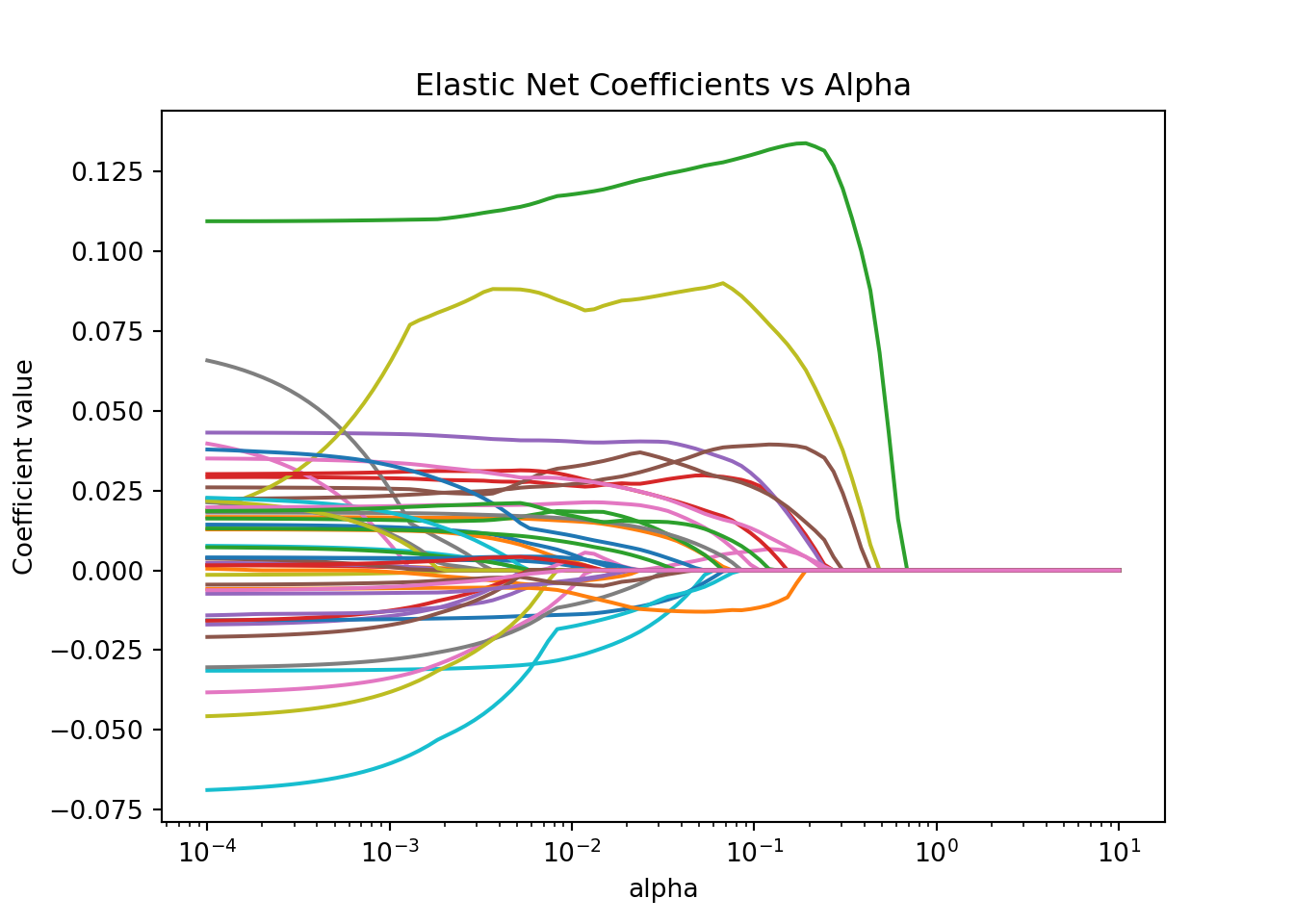
Here is a visual of the impact of adding more bias on the coefficients from our Ames housing model using an elastic net regression:
In a Jupyter environment, please rerun this cell to show the HTML representation or trust the notebook. On GitHub, the HTML representation is unable to render, please try loading this page with nbviewer.org.
Notice in the above plot that as the bias (represented by the x-axis) gets larger, the coefficients get closer to 0. Elastic net models blend together the penalties from both the ridge and LASSO regressions. That means that variables get zeroed out in their impact (by zeroing out the coefficients) just like in LASSO, but the curves are slightly smoother like in ridge.
Optimizing Penalties
In regularized regression models there is a fear of overfitting. We need to select the best value for our tuning parameter in our penalties, \(\lambda\). We don’t want the bias to be so high that we minimize variance to the point of overfitting our data and not making the model a good generalization of the overall pattern in the data.
As discussed in previous sections, cross-validation is a common approach to prevent overfitting when tuning a model parameter - here \(\lambda\). As a brief refresher, the concept of cross-validation is to:
Split training data into multiple pieces
Build model of majority of pieces
Evaluate model on remaining piece
Repeat process with switching out pieces for building and evaluation
Both ridge and LASSO regressions only have one parameter to tune - the bias penalty. However, elastic net regression has two parameters to tune, the bias penalty as well as the balance between the ridge and LASSO penalties. Due to the ridge and LASSO being special cases of the elastic net, it is sometimes easier to start off by optimizing the elastic net model first. If the ridge or LASSO appears to be the best option within the elastic net optimization, then we can fit one of those models.
Let’s see how to build these models in each software!
Let’s build a regularized regression for our Ames dataset. First, we must standardize our data. This is important so that all of the variables are on the same scale before adjustments are made to the estimated coefficients.
Instead of trying to decide ahead of time whether a ridge, LASSO, or Elastic net regression would be better for our data, we will let that balance be part of the tuning for our model. We will use the ElasticNetCV function from sklearn. We specify a 10-fold cross-validation using the cv = 10 option. The l1ratio option is looking at the balance of the two penalties as described above. We will test values between 0.001 (very closer to ridge regression) to 1 (LASSO regression). The ElasticNetCV function cannot actually provide an exact ridge regression, but we can get close. We will also test different levels of the \(\lambda\) penalty using the alphas option where we specify that we want it to test 100 different values. The naming conventions in the options are a little different than the equations above, but the idea remains the same.
Code
from sklearn.linear_model import ElasticNetCVfrom sklearn.preprocessing import StandardScaler# Standardize all variablesscaler = StandardScaler()X_reduced_standard = scaler.fit_transform(X_reduced)X_reduced_standard = pd.DataFrame(X_reduced_standard, columns = X_reduced.columns, index = X_reduced.index)# Set up ElasticNetCV with a grid of alphas and l1_ratioselastic_cv = ElasticNetCV( alphas=np.logspace(-4, 4, 100), # range of alpha (lambda) values l1_ratio=[0.001, 0.01, 0.1, 0.5, 0.7, 0.9, 1.0], # try different L1 ratios cv=10, random_state=1234, max_iter=100000)# Fit the modelelastic_cv.fit(X_reduced_standard, y_log)
In a Jupyter environment, please rerun this cell to show the HTML representation or trust the notebook. On GitHub, the HTML representation is unable to render, please try loading this page with nbviewer.org.
Parameters
l1_ratio
[0.001, 0.01, ...]
eps
0.001
n_alphas
'deprecated'
alphas
array([1.0000...00000000e+04])
fit_intercept
True
precompute
'auto'
max_iter
100000
tol
0.0001
cv
10
copy_X
True
verbose
0
n_jobs
None
positive
False
random_state
1234
selection
'cyclic'
Code
# Best parametersprint(f"Best alpha (lambda): {elastic_cv.alpha_:.5f}")
Best alpha (lambda): 0.29836
Code
print(f"Best l1_ratio: {elastic_cv.l1_ratio_}")
Best l1_ratio: 0.001
As we can see at the bottom of the output above by inspecting the alpha_ and l1_ratio_ elements, the optimal model has a penalty term of 0.29836 and l1_ratio of 0.001. With an l1_ratio this close to 0, it might be best to build a ridge regression model instead. Since the penalty term is also close to 0, this could easily be signaling that our OLS linear regression might be the best answer to this problem. However, let’s try the ridge regression approach anyway.
To build the ridge regression in Python we can use the RidgeCV function from sklearn as well. We will take the same approach we did with the elastic net model in standardizing our data first. We will search along the same grid for our penalty term as we did previously but no longer need to worry about optimizing a balance between ridge and LASSO penalties. The score_ function at the end of the code provides the model’s \(R^2\) value on the training data.
Code
from sklearn.linear_model import RidgeCV# Set up ElasticNetCV with a grid of alphas ridge_cv = RidgeCV( alphas=np.logspace(-4, 4, 100), # range of alpha (lambda) values cv=10)# Fit the modelridge_cv.fit(X_reduced_standard, y_log)
In a Jupyter environment, please rerun this cell to show the HTML representation or trust the notebook. On GitHub, the HTML representation is unable to render, please try loading this page with nbviewer.org.
Parameters
alphas
array([1.0000...00000000e+04])
fit_intercept
True
scoring
None
cv
10
gcv_mode
None
store_cv_results
False
alpha_per_target
False
Code
# Best parametersprint(f"Best alpha (lambda): {ridge_cv.alpha_:.5f}")
Best alpha (lambda): 422.92429
Code
# Model Metricr2 = ridge_cv.score(X_reduced_standard, y_log)print("R-squared:", r2)
R-squared: 0.8483663770623087
From the output above we see a different optimized value for the best penalty term than when we optimized with the ElasticNetCV function in the previous code. This could easily be due to the LASSO penalty, even as small as it was, impacting the optimization of the ridge penalty term.
Let’s build a regularized regression for our Ames dataset. Instead of trying to decide ahead of time whether a ridge, LASSO, or Elastic net regression would be better for our data, we will let that balance be part of the tuning for our model. We will use the same train function as before. Now we will use the method = "glmnet" option to build a regularized regression. Inside of our tuneGrid option we have multiple things to tune. The expand.grid function will fill in all of the combinations of values we want to tune. The .alpha = option is looking at the balance of the two penalties as described above. We will test values between 0 (ridge regression) to 1 (LASSO regression) by values of 0.05. We will also test different levels of the \(\lambda\) penalty using the .lambda = option. The trControl option stays the same to allow us to tune these models using 10-fold cross-validation.
Code
library(caret)data_combined <-data.frame(y_log = y_log, X_reduced)set.seed(1234)elastic_cv <- caret::train(y_log ~ ., data = data_combined,method ="glmnet", tuneGrid =expand.grid(.alpha =seq(0,1, by =0.05),.lambda =seq(0,25, by =0.1)), trControl =trainControl(method ='cv', number =10))elastic_cv$bestTune
  alpha lambda
1     0      0
As we can see at the bottom of the output above with the bestTune option, the optimal model has an \(\alpha = 0.5\) and \(\lambda = 100\). With an \(\alpha\) of 0, it might be best to build a ridge regression model instead. Since the penalty term is also 0, this could easily be signaling that our OLS linear regression might be the best answer to this problem. However, let’s try the ridge regression approach anyway.
In R, the cv.glmnet function will automatically implement a 10-fold CV (by default, but can be adjusted through options) to help evaluate and optimize the \(\lambda\) values for our regularized regression models at a finer tune than the train function of caret. However, the cv.glmnet function will not optimize the balance between the ridge and LASSO penalties like the train function.
We will build a ridge regression with \(\alpha = 0\) that we determined from the previous tuning. To build a model with the glmnet package we need separate data matrices for our predictors and our target variable with the x = option where we specify the predictor model matrix and the y = option where we specify the target variable. The alpha = 0 option specifies that a ridge regression will be used. The plot function allows us to see the impact of the penalty on the coefficients in the model.
The cv.glmnet function automatically standardizes the variables before fitting the regression model. This is important so that all of the variables are on the same scale before adjustments are made to the estimated coefficients.
Code
library(glmnet)set.seed(1234)X_reduced_mm <-model.matrix(y_log ~ ., data = data_combined)[, -1]ridge_cv <-cv.glmnet(x = X_reduced_mm, y =as.numeric(y_log), alpha =0)plot(ridge_cv)
Code
ridge_cv$lambda.min
[1] 0.1452876
Code
ridge_cv$lambda.1se
[1] 1.024976
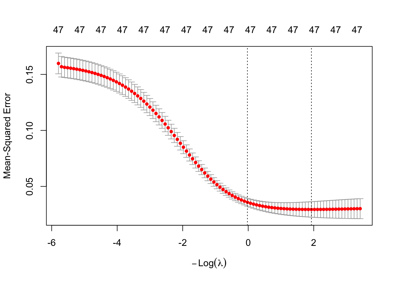
The above plot shows the results from our cross-validation. Here the models are evaluated based on their mean-squared error (MSE). The MSE is defined as \(\frac{1}{n} \sum_{i=1}^n (y_i - \hat{y}_i)^2\). The \(\lambda\) value that minimizes the MSE is 0.1452876 (with a \(\log(\lambda)\) = -1.929). This is highlighted by the first, vertical dashed line. The second vertical dashed line is the largest \(\lambda\) value that is one standard error above the minimum value. This value is especially useful in LASSO or elastic net regressions. The largest \(\lambda\) within one standard error would provide approximately the same MSE, but with a further reduction in the number of variables. However, in ridge regression it is not helpful since we are not reduced variables. Again, this low value of a penalty would signal that our original OLS linear regression might be the best solution.
Comparing Predictions
Models are nothing but potentially complicated formulas or rules. Once we determine the optimal model, we can score any new observations we want with the equation.
Scoring
It’s the process of applying a fitted model to input data to generate outputs like predicted values, probabilities, classifications, or scores.
Scoring data does not mean that we are re-running the model/algorithm on this new data. It just means that we are asking the model for predictions on this new data - plugging the new data into the equation and recording the output. This means that our data must be in the same format as the data put into the model. Therefore, if you created any new variables, made any variable transformations, or imputed missing values, the same process must be taken with the new data you are about to score.
For this problem we will score our test dataset that we have previously set aside as we were building our model. The test dataset is for comparing final models and reporting final model metrics. Make sure that you do NOT go back and rebuild your model after you score the test dataset. This would no longer make the test dataset an honest assessment of how good your model is actually doing. That also means that we should NOT just build hundreds of iterations of our same model to compare to the test dataset. That would essentially be doing the same thing as going back and rebuilding the model as you would be letting the test dataset decide on your final model.
Without going into all of the same detail as before, the following code transforms the test dataset we originally created in the same way that we did for the training dataset by dropping necessary variables, making missing value imputations, and getting our same data objects.
Code
import statsmodels.api as smpredictors_test = test.drop(columns=['SalePrice'])ames_dummied = pd.get_dummies(ames, drop_first=True)test_ids = test.indextest_dummied = ames_dummied.loc[test_ids]predictors_test = test_dummied.astype(float)predictors_test = predictors_test.drop(['GarageType_Missing', 'GarageQual_Missing','GarageCond_Missing'], axis=1)# Impute Missing for Continuous Variablesnum_cols = predictors_test.select_dtypes(include='number').columnsfor col in num_cols:if predictors_test[col].isnull().any():# Create missing flag column predictors_test[f'{col}_was_missing'] = predictors_test[col].isnull().astype(int)# Impute with median median = predictors_test[col].median() predictors_test[col] = predictors_test[col].fillna(median)X_test = predictors_testy_test = test['SalePrice']y_test_log = np.log(test['SalePrice'])# Subset the DataFrame to selected featuresX_test_selected = X_test[selected_features].copy()X_test_selected = sm.add_constant(X_test_selected)
Now that our data is ready for scoring we can use the predict function on our model object we created with our previous linear regression with stepwise selection variables on the natural log of the target variable. The only input to the predict function is the dataset we prepared for scoring. Since the predictions will be in the same natural log form as the model, we use the np.exp function to transform our predictions back to their original scale of sale price in dollars.
From the sklearn.metrics package we have a variety of model metric functions. We will use the mean_absolute_error (MAE) and mean_absolute_percentage_error (MAPE) metrics like the ones we described in the section on Model Building.
From the above output we can see that the linear regression model beats the ridge regression model. This isn’t too surprising as there were signs in the above optimization of the elastic net model that our OLS linear regression might be the best solution.
Model
MAE
MAPE
Linear Regression
$18,160.24
11.36%
Ridge Regression
$19.572.19
12.25%
To help ensure that the transformations are the same between both Python and R, I am just importing my Python objects into R to get the same datasets.
Now that our data is ready for scoring we can use the predict function on our model object we created with our previous linear regression with stepwise selection variables on the natural log of the target variable. The only inputs to the predict function are the model object you want to use to score and the new dataset we prepared for scoring. Since the predictions will be in the same natural log form as the model, we use the exp function to transform our predictions back to their original scale of sale price in dollars.
We then calculate the mean absolute error (MAE) and mean absolute percentage error (MAPE) metrics like the ones we described in the section on Model Building.
From the above output we can see that the linear regression model beats the ridge regression model. This isn’t too surprising as there were signs in the above optimization of the elastic net model that our OLS linear regression might be the best solution.
Model
MAE
MAPE
Linear Regression
$18,160.24
11.36%
Ridge Regression
$22,040.76
13.37%
Source Code
---title: "Regularized Regression"format: html: code-fold: show code-tools: trueengine: knitreditor: visual---```{r}#| include: false#| warning: false#| error: false#| message: falselibrary(reticulate)reticulate::use_condaenv("wfu_fall_ml", required =TRUE)``````{python}#| include: false#| warning: false#| error: false#| message: falsefrom sklearn.datasets import fetch_openmlimport pandas as pdfrom sklearn.feature_selection import SelectKBest, f_classifimport numpy as npimport matplotlib.pyplot as plt# Load Ames Housing datadata = fetch_openml(name="house_prices", as_frame=True)ames = data.frame# Remove Business Logic Variablesames = ames.drop(['Id', 'MSSubClass','Functional','MSZoning','Neighborhood', 'LandSlope','Condition2','OverallCond','RoofStyle','RoofMatl','Exterior1st','Exterior2nd','MasVnrType','MasVnrArea','ExterCond','BsmtCond','BsmtExposure','BsmtFinType1','BsmtFinSF1','BsmtFinType2','BsmtFinSF2','BsmtUnfSF','Electrical','LowQualFinSF','BsmtFullBath','BsmtHalfBath','KitchenAbvGr','GarageFinish','SaleType','SaleCondition'], axis=1)# Remove Missingness Variablesames = ames.drop(['PoolQC', 'MiscFeature','Alley', 'Fence'], axis=1)# Impute Missingness for Categorical Variablescat_cols = ames.select_dtypes(include=['object', 'category']).columnsames[cat_cols] = ames[cat_cols].fillna('Missing')# Remove Low Variability Variablesames = ames.drop(['Street', 'Utilities','Heating'], axis=1)# Train / Test Splitfrom sklearn.model_selection import train_test_splittrain, test = train_test_split(ames, test_size =0.25, random_state =1234)# Impute Missing for Continuous Variablesnum_cols = train.select_dtypes(include='number').columnsfor col in num_cols:if train[col].isnull().any():# Create missing flag column train[f'{col}_was_missing'] = train[col].isnull().astype(int)# Impute with median median = train[col].median() train[col] = train[col].fillna(median)# Prepare X and y Objectsimport statsmodels.api as smpredictors = train.drop(columns=['SalePrice'])predictors = pd.get_dummies(predictors, drop_first=True)predictors = predictors.astype(float)predictors = predictors.drop(['GarageType_Missing', 'GarageQual_Missing','GarageCond_Missing'], axis=1)X = predictorsy = train['SalePrice']y_log = np.log(train['SalePrice'])# Initial Variable Selectionselector = SelectKBest(score_func=f_classif, k='all') selector.fit(X, y)pval_df = pd.DataFrame({'Feature': X.columns,'F_score': selector.scores_,'p_value': selector.pvalues_})selected_features = pval_df[pval_df['p_value'] <0.009]['Feature']X_reduced = X[selected_features.tolist()]# Stepwise Selectionfrom mlxtend.feature_selection import SequentialFeatureSelector as SFSfrom sklearn.linear_model import LinearRegression# Modellr = LinearRegression()# Stepwise selection to find best number of featuressfs = SFS(lr, k_features="best", forward=True, floating=True, scoring='neg_mean_squared_error', cv=10)sfs = sfs.fit(X_reduced, y_log)# Get selected feature namesselected_features =list(sfs.k_feature_names_)X_selected = X_reduced[selected_features].copy()``````{r}#| include: false#| warning: false#| error: false#| message: falsetrain = py$traintest = py$testX_selected = py$X_selectedX_reduced = py$X_reducedy = py$yy_log = py$y_log```# RegularizationLinear regression is a great initial approach to take to model building. In fact, in the realm of statistical models, linear regression (calculated by ordinary least squares) is the **best linear unbiased estimator**. The two key pieces to that previous statement are "best" and "unbiased."What does it mean to be **unbiased**? Each of the sample coefficients ($\hat{\beta}$'s) in the regression model are estimates of the true coefficients. These sample coefficients have sampling distributions - specifically, normally distributed sampling distributions. The mean of the sampling distribution of $\hat{\beta}_j$ is the true (unknown) coefficient $\beta_j$. This means the coefficient is unbiased.What does it mean to be **best**? *IF* the assumptions of ordinary least squares are met fully, then the sampling distributions of the coefficients in the model have the **minimum** variance of all **unbiased** estimators.These two things combined seem like what we want in a model - estimating what we want (unbiased) and doing it in a way that has the minimum amount of variation (best among the unbiased). Again, these rely on the assumptions of linear regression holding true. Another approach to regression would be to use **regularized regression** instead as a different approach to building the model.As the number of variables in a linear regression model increase, the chances of having a model that meets all of the assumptions starts to diminish. Multicollinearity can also pose a large problem with bigger regression models. The coefficients of a linear regression vary widely in the presence of multicollinearity. These variations lead to over-fitting of a regression model. More formally, these models have higher variance than desired. In those scenarios, moving out of the realm of unbiased estimates may provide a lower variance in the model, even though the model is no longer unbiased as described above. We wouldn't want to be too biased, but some small degree of bias might improve the model's fit overall and even lead to better predictions at the cost of a lack of interpretability.Another potential problem for linear regression is when we have more variables than observations in our data set. This is a common problem in the space of genetic modeling. In this scenario, the ordinary least squares approach leads to multiple solutions instead of just one. Unfortunately, most of these infinite solutions over-fit the problem at hand anyway.Regularized (or **penalized** or **shrinkage**) regression techniques potentially alleviate these problems. Regularized regression puts constraints on the estimated coefficients in our model and *shrink* these estimates to zero. This helps reduce the variation in the coefficients (improving the variance of the model), but at the cost of biasing the coefficients. The specific constraints that are put on the regression inform the three common approaches - **ridge regression**, **LASSO**, and **elastic nets**.## Penalties in ModelsIn ordinary least squares linear regression, we minimize the sum of the squared residuals (or errors).$$min(\sum_{i=1}^n(y_i - \hat{y}_i)^2) = min(SSE)$$In regularized regression, however, we add a penalty term to the $SSE$ as follows:$$min(\sum_{i=1}^n(y_i - \hat{y}_i)^2 + Penalty) = min(SSE + Penalty)$$As mentioned above, the penalties we choose constrain the estimated coefficients in our model and shrink these estimates to zero. Different penalties have different effects on the estimated coefficients. Two common approaches to adding penalties are the ridge and LASSO approaches. The elastic net approach is a combination of these two. Let's explore each of these in further detail.## Ridge RegressionRidge regression adds what is commonly referred to as an "$L_2$" penalty:$$min(\sum_{i=1}^n(y_i - \hat{y}_i)^2 + \lambda \sum_{j=1}^p \hat{\beta}^2_j) = min(SSE + \lambda \sum_{j=1}^p \hat{\beta}^2_j)$$This penalty is controlled by the **tuning parameter** $\lambda$. If $\lambda = 0$, then we have typical OLS linear regression. However, as $\lambda \rightarrow \infty$, the coefficients in the model shrink to zero. This makes intuitive sense. Since the estimated coefficients, $\hat{\beta}_j$'s, are the only thing changing to minimize this equation, then as $\lambda \rightarrow \infty$, the equation is best minimized by forcing the coefficients to be smaller and smaller. We will see how to optimize this penalty term later in this section.Here is a visual of the impact of adding more bias on the coefficients from our Ames housing model using a ridge regression:```{python}#| warning: false#| error: false#| message: false#| echo: false#| results: 'hide'from sklearn.linear_model import Ridgefrom sklearn.linear_model import Lassofrom sklearn.linear_model import ElasticNetfrom sklearn.preprocessing import StandardScaler# Standardize all variablesscaler = StandardScaler()X_reduced_standard = scaler.fit_transform(X_reduced)X_reduced_standard = pd.DataFrame(X_reduced_standard, columns = X_reduced.columns, index = X_reduced.index)model_ridge = Ridge(alpha =1.0).fit(X_reduced_standard, y_log)None``````{python}#| warning: false#| error: false#| message: false#| echo: falsen_alphas =200alphas = np.logspace(0.1, 6, n_alphas)coefs = []for a in alphas: ridge = Ridge(alpha=a) ridge.fit(X_reduced_standard, y_log) coefs.append(ridge.coef_)plt.cla()ax = plt.gca()ax.plot(alphas, coefs)ax.set_xscale("log")plt.xlabel("alpha")plt.ylabel("weights")plt.title("Ridge coefficients as a function of the regularization")plt.axis("tight")plt.show()```Notice in the above plot that as the bias (represented by the x-axis) gets larger, the coefficients get closer to 0. However, those coefficients are asymptotically approaching 0 while never equaling it. This is different than the next approach!## LASSO**Least absolute shrinkage and selection operator** (LASSO) regression adds what is commonly referred to as an "$L_1$" penalty:$$min(\sum_{i=1}^n(y_i - \hat{y}_i)^2 + \lambda \sum_{j=1}^p |\hat{\beta}_j|) = min(SSE + \lambda \sum_{j=1}^p |\hat{\beta}_j|)$$This penalty is controlled by the **tuning parameter** $\lambda$. If $\lambda = 0$, then we have typical OLS linear regression. However, as $\lambda \rightarrow \infty$, the coefficients in the model shrink to zero. This makes intuitive sense. Since the estimated coefficients, $\hat{\beta}_j$'s, are the only thing changing to minimize this equation, then as $\lambda \rightarrow \infty$, the equation is best minimized by forcing the coefficients to be smaller and smaller. We will see how to optimize this penalty term later in this section.However, unlike ridge regression that has the coefficient estimates approach zero asymptotically, in LASSO regression the coefficients can actually equal zero. This may not be as intuitive when initially looking at the penalty terms themselves. It becomes easier to see when dealing with the solutions to the coefficient estimates. Without going into too much mathematical detail, this is done by taking the derivative of the minimization function (objective function) and setting it equal to zero. From there we can determine the optimal solution for the estimated coefficients. In OLS regression the estimates for the coefficients can be shown to equal the following (in matrix form):$$\hat{\beta} = (X^TX)^{-1}X^TY$$This changes in the presence of penalty terms. For ridge regression, the solution becomes the following:$$\hat{\beta} = (X^TX + \lambda I)^{-1}X^TY$$There is no value for $\lambda$ that can force the coefficients to be zero by itself. Therefore, unless the data makes the coefficient zero, the penalty term can only force the estimated coefficient to zero asymptotically as $\lambda \rightarrow \infty$.However, for LASSO, the solution isn't quite as easy to show. However, in this scenario, there is a possible penalty value that will force the estimated coefficients to equal zero. There is some benefit to this. This makes LASSO also function as a variable selection criteria as well.Here is a visual of the impact of adding more bias on the coefficients from our Ames housing model using a LASSO regression:```{python}#| warning: false#| error: false#| message: false#| include: falsemodel_lasso = Lasso(alpha =0.01, max_iter =5000).fit(X_reduced_standard, y_log);``````{python}#| warning: false#| error: false#| message: false#| echo: falsen_alphas =100alphas2 = np.logspace(-4,0, n_alphas)coefs2 = []for a in alphas2: lasso = Lasso(alpha = a, max_iter =5000) lasso.fit(X_reduced_standard, y_log) coefs2.append(lasso.coef_)plt.cla()ax2 = plt.gca()ax2.plot(alphas2, coefs2)ax2.set_xscale("log")plt.xlabel("alpha")plt.ylabel("weights")plt.title("LASSO coefficients as a function of the regularization")plt.axis("tight")plt.show()```Notice in the above plot that as the bias (represented by the x-axis) gets larger, the coefficients get closer to 0. However, unlike ridge regression, there comes a point where a coefficient effectively gets zeroed out. Once that coefficient gets zeroed out, the model no longer is impacted by that variable which essentially removes the variable from the model.## Elastic NetWhich approach is better, ridge or LASSO? Both have advantages and disadvantages. LASSO performs variable selection while ridge keeps all variables in the model. However, reducing the number of variables might impact minimum error. Also, if you have two correlated variables, which one LASSO chooses to zero out is relatively arbitrary to the context of the problem.Elastic nets were designed to take advantage of both penalty approaches. In elastic nets, we are using both penalties in the minimization:$$min(SSE + \lambda_1 \sum_{j=1}^p |\hat{\beta}_j| + \lambda_2 \sum_{j=1}^p \hat{\beta}^2_j) $$Both R and Python take a slightly different approach to the elastic net implementation with the following:$$min(SSE + \alpha[ \rho \sum_{j=1}^p |\hat{\beta}_j| + (1-\rho) \sum_{j=1}^p \hat{\beta}^2_j]) $$They still have one penalty $\alpha$, however, it includes the $\rho$ parameter to balance between the two penalty terms. Any value in between zero and one will provide an elastic net.Here is a visual of the impact of adding more bias on the coefficients from our Ames housing model using an elastic net regression:```{python}#| warning: false#| error: false#| message: false#| include: falsemodel_en = ElasticNet(alpha =0.01, l1_ratio=0.5).fit(X_reduced_standard, y_log);``````{python}#| warning: false#| error: false#| message: false#| echo: falsealphas3 = np.logspace(-4, 1, 100) coefs = []for alpha in alphas3: en = ElasticNet(alpha=alpha, l1_ratio=0.5, max_iter=10000) en.fit(X_reduced_standard, y_log) coefs.append(en.coef_)coefs = np.array(coefs)plt.cla()for i inrange(coefs.shape[1]): plt.plot(alphas3, coefs[:, i], label=f'X{i}'if X.columns isNoneelse X.columns[i])plt.xscale('log')plt.xlabel('alpha')plt.ylabel('Coefficient value')plt.title('Elastic Net Coefficients vs Alpha')plt.axis('tight')plt.show()```Notice in the above plot that as the bias (represented by the x-axis) gets larger, the coefficients get closer to 0. Elastic net models blend together the penalties from both the ridge and LASSO regressions. That means that variables get zeroed out in their impact (by zeroing out the coefficients) just like in LASSO, but the curves are slightly smoother like in ridge.# Optimizing PenaltiesIn regularized regression models there is a fear of overfitting. We need to select the best value for our tuning parameter in our penalties, $\lambda$. We don't want the bias to be so high that we minimize variance to the point of overfitting our data and not making the model a good generalization of the overall pattern in the data.As discussed in previous sections, **cross-validation** is a common approach to prevent overfitting when tuning a model parameter - here $\lambda$. As a brief refresher, the concept of cross-validation is to:- Split training data into [multiple]{.underline} pieces- Build model of [majority]{.underline} of pieces- Evaluate model on [remaining]{.underline} piece- Repeat process with [switching]{.underline} out pieces for building and evaluationBoth ridge and LASSO regressions only have one parameter to tune - the bias penalty. However, elastic net regression has two parameters to tune, the bias penalty as well as the balance between the ridge and LASSO penalties. Due to the ridge and LASSO being special cases of the elastic net, it is sometimes easier to start off by optimizing the elastic net model first. If the ridge or LASSO appears to be the best option within the elastic net optimization, then we can fit one of those models.Let's see how to build these models in each software!::: {.panel-tabset .nav-pills}## PythonLet's build a regularized regression for our Ames dataset. First, we must standardize our data. This is important so that all of the variables are on the same scale before adjustments are made to the estimated coefficients.Instead of trying to decide ahead of time whether a ridge, LASSO, or Elastic net regression would be better for our data, we will let that balance be part of the tuning for our model. We will use the `ElasticNetCV` function from `sklearn`. We specify a 10-fold cross-validation using the `cv = 10` option. The `l1ratio` option is looking at the balance of the two penalties as described above. We will test values between 0.001 (very closer to ridge regression) to 1 (LASSO regression). The `ElasticNetCV` function cannot actually provide an exact ridge regression, but we can get close. We will also test different levels of the $\lambda$ penalty using the `alphas` option where we specify that we want it to test 100 different values. The naming conventions in the options are a little different than the equations above, but the idea remains the same.```{python}#| warning: false#| error: false#| message: falsefrom sklearn.linear_model import ElasticNetCVfrom sklearn.preprocessing import StandardScaler# Standardize all variablesscaler = StandardScaler()X_reduced_standard = scaler.fit_transform(X_reduced)X_reduced_standard = pd.DataFrame(X_reduced_standard, columns = X_reduced.columns, index = X_reduced.index)# Set up ElasticNetCV with a grid of alphas and l1_ratioselastic_cv = ElasticNetCV( alphas=np.logspace(-4, 4, 100), # range of alpha (lambda) values l1_ratio=[0.001, 0.01, 0.1, 0.5, 0.7, 0.9, 1.0], # try different L1 ratios cv=10, random_state=1234, max_iter=100000)# Fit the modelelastic_cv.fit(X_reduced_standard, y_log)# Best parametersprint(f"Best alpha (lambda): {elastic_cv.alpha_:.5f}")print(f"Best l1_ratio: {elastic_cv.l1_ratio_}")```As we can see at the bottom of the output above by inspecting the `alpha_` and `l1_ratio_` elements, the optimal model has a penalty term of 0.29836 and `l1_ratio` of 0.001. With an `l1_ratio` this close to 0, it might be best to build a ridge regression model instead. Since the penalty term is also close to 0, this could easily be signaling that our OLS linear regression might be the best answer to this problem. However, let's try the ridge regression approach anyway.To build the ridge regression in Python we can use the `RidgeCV` function from `sklearn` as well. We will take the same approach we did with the elastic net model in standardizing our data first. We will search along the same grid for our penalty term as we did previously but no longer need to worry about optimizing a balance between ridge and LASSO penalties. The `score_` function at the end of the code provides the model's $R^2$ value on the training data.```{python}#| warning: false#| error: false#| message: falsefrom sklearn.linear_model import RidgeCV# Set up ElasticNetCV with a grid of alphas ridge_cv = RidgeCV( alphas=np.logspace(-4, 4, 100), # range of alpha (lambda) values cv=10)# Fit the modelridge_cv.fit(X_reduced_standard, y_log)# Best parametersprint(f"Best alpha (lambda): {ridge_cv.alpha_:.5f}")# Model Metricr2 = ridge_cv.score(X_reduced_standard, y_log)print("R-squared:", r2)```From the output above we see a different optimized value for the best penalty term than when we optimized with the `ElasticNetCV` function in the previous code. This could easily be due to the LASSO penalty, even as small as it was, impacting the optimization of the ridge penalty term.## RLet's build a regularized regression for our Ames dataset. Instead of trying to decide ahead of time whether a ridge, LASSO, or Elastic net regression would be better for our data, we will let that balance be part of the tuning for our model. We will use the same `train` function as before. Now we will use the `method = "glmnet"` option to build a regularized regression. Inside of our `tuneGrid` option we have multiple things to tune. The `expand.grid` function will fill in all of the combinations of values we want to tune. The `.alpha =` option is looking at the balance of the two penalties as described above. We will test values between 0 (ridge regression) to 1 (LASSO regression) by values of 0.05. We will also test different levels of the $\lambda$ penalty using the `.lambda =` option. The `trControl` option stays the same to allow us to tune these models using 10-fold cross-validation.```{r}#| warning: false#| error: false#| message: falselibrary(caret)data_combined <-data.frame(y_log = y_log, X_reduced)set.seed(1234)elastic_cv <- caret::train(y_log ~ ., data = data_combined,method ="glmnet", tuneGrid =expand.grid(.alpha =seq(0,1, by =0.05),.lambda =seq(0,25, by =0.1)), trControl =trainControl(method ='cv', number =10))elastic_cv$bestTune```As we can see at the bottom of the output above with the `bestTune` option, the optimal model has an $\alpha = 0.5$ and $\lambda = 100$. With an $\alpha$ of 0, it might be best to build a ridge regression model instead. Since the penalty term is also 0, this could easily be signaling that our OLS linear regression might be the best answer to this problem. However, let's try the ridge regression approach anyway.In R, the `cv.glmnet` function will automatically implement a 10-fold CV (by default, but can be adjusted through options) to help evaluate and optimize the $\lambda$ values for our regularized regression models at a finer tune than the `train` function of `caret`. However, the `cv.glmnet` function will **not** optimize the balance between the ridge and LASSO penalties like the `train` function.We will build a ridge regression with $\alpha = 0$ that we determined from the previous tuning. To build a model with the `glmnet` package we need separate data matrices for our predictors and our target variable with the `x =` option where we specify the predictor model matrix and the `y =` option where we specify the target variable. The `alpha = 0` option specifies that a ridge regression will be used. The `plot` function allows us to see the impact of the penalty on the coefficients in the model.The `cv.glmnet` function automatically standardizes the variables before fitting the regression model. This is important so that all of the variables are on the same scale before adjustments are made to the estimated coefficients.```{r}#| warning: false#| error: false#| message: falselibrary(glmnet)set.seed(1234)X_reduced_mm <-model.matrix(y_log ~ ., data = data_combined)[, -1]ridge_cv <-cv.glmnet(x = X_reduced_mm, y =as.numeric(y_log), alpha =0)plot(ridge_cv)ridge_cv$lambda.minridge_cv$lambda.1se```The above plot shows the results from our cross-validation. Here the models are evaluated based on their **mean-squared error** (MSE). The MSE is defined as $\frac{1}{n} \sum_{i=1}^n (y_i - \hat{y}_i)^2$. The $\lambda$ value that minimizes the MSE is 0.1452876 (with a $\log(\lambda)$ = -1.929). This is highlighted by the first, vertical dashed line. The second vertical dashed line is the largest $\lambda$ value that is one standard error above the minimum value. This value is especially useful in LASSO or elastic net regressions. The largest $\lambda$ within one standard error would provide approximately the same MSE, but with a further reduction in the number of variables. However, in ridge regression it is not helpful since we are not reduced variables. Again, this low value of a penalty would signal that our original OLS linear regression might be the best solution.:::# Comparing PredictionsModels are nothing but potentially complicated formulas or rules. Once we determine the optimal model, we can **score** any new observations we want with the equation.::: callout-tip## ScoringIt's the process of applying a fitted model to input data to generate outputs like predicted values, probabilities, classifications, or scores.:::Scoring data **does not** mean that we are re-running the model/algorithm on this new data. It just means that we are asking the model for predictions on this new data - plugging the new data into the equation and recording the output. This means that our data must be in the same format as the data put into the model. Therefore, if you created any new variables, made any variable transformations, or imputed missing values, the same process must be taken with the new data you are about to score.For this problem we will score our test dataset that we have previously set aside as we were building our model. The test dataset is for comparing final models and reporting final model metrics. Make sure that you do **NOT** go back and rebuild your model after you score the test dataset. This would no longer make the test dataset an honest assessment of how good your model is actually doing. That also means that we should **NOT** just build hundreds of iterations of our same model to compare to the test dataset. That would essentially be doing the same thing as going back and rebuilding the model as you would be letting the test dataset decide on your final model.Let's score our data in each software!::: {.panel-tabset .nav-pills}## PythonWithout going into all of the same detail as before, the following code transforms the test dataset we originally created in the same way that we did for the training dataset by dropping necessary variables, making missing value imputations, and getting our same data objects.```{python}#| warning: false#| error: false#| message: falseimport statsmodels.api as smpredictors_test = test.drop(columns=['SalePrice'])ames_dummied = pd.get_dummies(ames, drop_first=True)test_ids = test.indextest_dummied = ames_dummied.loc[test_ids]predictors_test = test_dummied.astype(float)predictors_test = predictors_test.drop(['GarageType_Missing', 'GarageQual_Missing','GarageCond_Missing'], axis=1)# Impute Missing for Continuous Variablesnum_cols = predictors_test.select_dtypes(include='number').columnsfor col in num_cols:if predictors_test[col].isnull().any():# Create missing flag column predictors_test[f'{col}_was_missing'] = predictors_test[col].isnull().astype(int)# Impute with median median = predictors_test[col].median() predictors_test[col] = predictors_test[col].fillna(median)X_test = predictors_testy_test = test['SalePrice']y_test_log = np.log(test['SalePrice'])# Subset the DataFrame to selected featuresX_test_selected = X_test[selected_features].copy()X_test_selected = sm.add_constant(X_test_selected)```Now that our data is ready for scoring we can use the `predict` function on our model object we created with our previous linear regression with stepwise selection variables on the natural log of the target variable. The only input to the `predict` function is the dataset we prepared for scoring. Since the predictions will be in the same natural log form as the model, we use the `np.exp` function to transform our predictions back to their original scale of sale price in dollars.From the `sklearn.metrics` package we have a variety of model metric functions. We will use the `mean_absolute_error` (MAE) and `mean_absolute_percentage_error` (MAPE) metrics like the ones we described in the section on Model Building.```{python}#| warning: false#| error: false#| message: falsefrom sklearn.metrics import mean_absolute_errorfrom sklearn.metrics import mean_absolute_percentage_errorX_selected = X_reduced[selected_features].copy()X_selected = sm.add_constant(X_selected)model = sm.OLS(y_log, X_selected).fit()lr_pred_log = model.predict(X_test_selected)lr_pred = np.exp(lr_pred_log)mae = mean_absolute_error(y_test, lr_pred)mape = mean_absolute_percentage_error(y_test, lr_pred)print(f"MAE: {mae:.2f}")print(f"MAPE: {mape:.2%}")```We can use the same logic and code structure to obtain the predictions from our ridge regression model as well.```{python}#| warning: false#| error: false#| message: falseX_test_reduced = X_test[X_reduced.columns].copy()scaler = StandardScaler()X_test_reduced_standard = scaler.fit_transform(X_test_reduced)X_test_reduced_standard = pd.DataFrame(X_test_reduced_standard, columns = X_test_reduced.columns, index = X_test_reduced.index)rr_pred_log = ridge_cv.predict(X_test_reduced_standard)rr_pred = np.exp(rr_pred_log)mae_r = mean_absolute_error(y_test, rr_pred)mape_r = mean_absolute_percentage_error(y_test, rr_pred)print(f"MAE: {mae_r:.2f}")print(f"MAPE: {mape_r:.2%}")```From the above output we can see that the linear regression model beats the ridge regression model. This isn't too surprising as there were signs in the above optimization of the elastic net model that our OLS linear regression might be the best solution.| Model | MAE | MAPE ||:-----------------:|:-----------:|:------:|| Linear Regression | \$18,160.24 | 11.36% || Ridge Regression | \$19.572.19 | 12.25% |## RTo help ensure that the transformations are the same between both Python and R, I am just importing my Python objects into R to get the same datasets.```{r}#| warning: false#| error: false#| message: falseX_test_selected = py$X_test_selectedX_test_reduced = py$X_test_reducedy_test = py$y_test```Now that our data is ready for scoring we can use the `predict` function on our model object we created with our previous linear regression with stepwise selection variables on the natural log of the target variable. The only inputs to the `predict` function are the model object you want to use to score and the new dataset we prepared for scoring. Since the predictions will be in the same natural log form as the model, we use the `exp` function to transform our predictions back to their original scale of sale price in dollars.We then calculate the mean absolute error (MAE) and mean absolute percentage error (MAPE) metrics like the ones we described in the section on Model Building.```{r}#| warning: false#| error: false#| message: falsemodel_lin <-lm(y_log ~ . , data = X_selected)lr_pred_log <-predict(model_lin, newdata = X_test_selected)lr_pred <-exp(lr_pred_log)mae <-mean(abs(lr_pred - y_test))mape <-mean(abs(lr_pred - y_test)/y_test)cat(sprintf("MAE: %.2f\n", mae))cat(sprintf("MAPE: %.2f%%\n", mape *100))```We can use the same logic and code structure to obtain the predictions from our ridge regression model as well.```{r}#| warning: false#| error: false#| message: falsedata_test_combined <-data.frame(y_test = y_test, X_test_reduced)X_test_reduced_mm <-model.matrix(y_test ~ ., data = data_test_combined)[, -1]rr_pred_log <-predict(ridge_cv, newx = X_test_reduced_mm)rr_pred <-exp(as.numeric(rr_pred_log))mae <-mean(abs(rr_pred - y_test))mape <-mean(abs(rr_pred - y_test)/y_test)cat(sprintf("MAE: %.2f\n", mae))cat(sprintf("MAPE: %.2f%%\n", mape *100))```From the above output we can see that the linear regression model beats the ridge regression model. This isn't too surprising as there were signs in the above optimization of the elastic net model that our OLS linear regression might be the best solution.| Model | MAE | MAPE ||:-----------------:|:-----------:|:------:|| Linear Regression | \$18,160.24 | 11.36% || Ridge Regression | \$22,040.76 | 13.37% |:::