Categorical Data Considerations

Introduction

There are a lot of considerations one should take with data involving a logistic regression. What happens if my event of interest is a rare occurrence in my data set? How do categorical variables influence the convergence of my logistic regression model? These are the important things we need to account for in modeling.

Rare Event Sampling

Classification models try to predict categorical target variables, typically where one of the categories is of main interest. What if this category of interest doesn’t happen frequently in the data set? This is referred to as rare-event modeling and exists in many fields such as fraud, credit default, marketing responses, and rare weather events. The typical cut-off people use to decide if their event is rare is 5%. If your event occurs less than 5% of the time, you should adjust your modeling to account for this.

We will be using the telecomm data set data set to model the association between various factors and a customer churning from the company. The variables in the data set are the following:

Variable	Description
account_length	length of time with company
international_plan	yes, no
voice_mail_plan	yes, no
customer_service_calls	number of service calls
total_day_minutes	minutes used during daytime
total_day_calls	calls used during daytime
total_day_charge	cost of usage during daytime
Same as previous 3 for evening, night, international	same as above

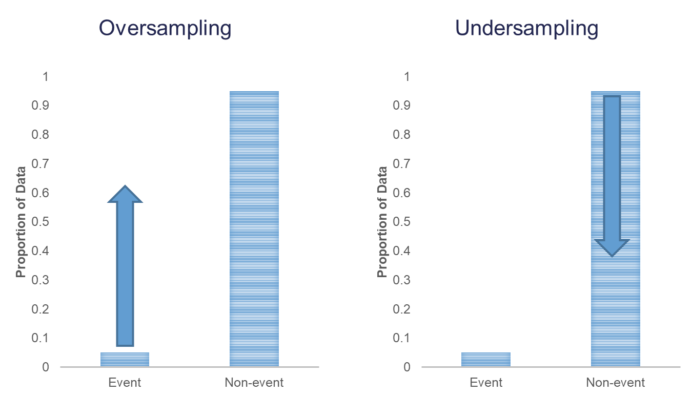
When you have a rare event situation, you can adjust for this by balancing out the sample in your training data set. This can be done through sampling techniques typically called oversampling. When oversampling, you can either over or under sample your target variable to get balance.

Oversampling is when you replicate your rare event enough times to balance out with your non-events in your training data sets. There are a variety of different ways to replicate observations, but for now we will only focus on true replication - copying our actual observations at random until we get balance. This will inflate our training data set size.

Undersampling is when we randomly sample only enough observations from the non-events in our training data set to balance out with events. This will make our training data set size much smaller. These are both represented in the following figure:

Let’s see how to perform these in each software!

Python
R

In Python we can easily perform both over and under sampling respectively. First, we examine the proportional breakdown of our target variable with the crosstab function divided by the sum of the rows in the table to get the proportions. Specifically we want to view the churn variable. We can see below that we have roughly 5% of the customers in our data churn from the company.

Code

pd.crosstab(index = telecomm['churn'], columns = "prop")/pd.crosstab(index = telecomm['churn'], columns = "prop").sum()

col_0      prop
churn          
False  0.948735
True   0.051265

It is easy to perform undersampling in Python with some basic data manipulation functions. Below we use the groupby function to group by our target variable churn. From the above output, we have 154 churners in our dataset. Let’s sample 104 of them for the training and leave the remaining 50 for testing. Now we just need a random sample of 104 of each of the churners and non-churners from our dataset. For this we use the sample function. The training data is defined as the rows that have these row indices and the test data set is defined as the rows that don’t have these indices.

Code

train_u = telecomm.groupby("churn").sample(n = 104, random_state = 1234)

test_u = telecomm.loc[telecomm.index.difference(train_u.index)]

The crosstab functions then show the number of observations in each data set for the churn variable.

Code

pd.crosstab(index = train_u['churn'], columns = "count")

col_0  count
churn       
False    104
True     104

Code

pd.crosstab(index = test_u['churn'], columns = "count")

col_0  count
churn       
False   2746
True      50

Oversampling is also easy to perform in Python. There are many ways to duplicate rows in Python. First, we use the sample function with the frac option to isolate down to 70% of the observations. From there we want to isolate the churners to replicate them. For this we create a new dataframe, is_churn, with churn equal to True. We then replicate this dataset 9 times and combine them together using the concat function.

Code

train_churn = telecomm.sample(frac = 0.7, random_state = 4321)
test_o = telecomm.drop(train_churn.index)

# Isolate Churners and Replicate
is_churn = train_churn['churn'] == True

concat_list = pd.concat([train_churn[is_churn]] * 9)

train_o =  pd.concat([train_churn, concat_list])

pd.crosstab(index = train_o['churn'], columns = "count")

col_0  count
churn       
False   1992
True    1110

Code

pd.crosstab(index = test_o['churn'], columns = "count")

col_0  count
churn       
False    858
True      43

In R we can easily perform both over and under sampling respectively. First, we examine the proportional breakdown of our target variable with the table and prop.table functions. Specifically we want to view the churn variable. We can see below that we have roughly 5% of the customers in our data churn from the company. We also create a new id variable in the dataset by simply starting with the number 1 and going through the length of the dataset.

Code

table(telecomm$churn)


FALSE  TRUE 
 2850   154

Code

prop.table(table(telecomm$churn))


     FALSE       TRUE 
0.94873502 0.05126498

Code

telecomm$id <- 1:length(telecomm$churn)

It is easy to perform undersampling in R with some basic data manipulation functions. Below we use the group_by function to group by our target variable churn. From the above output, we have 154 churners in our dataset. Let’s sample 104 of them for the training and leave the remaining 50 for testing. Now we just need a random sample of 104 of each of the churners and non-churners from our dataset. For this we use the sample_n function. The training data is defined as the rows that have these row ID’s and the test data set is defined as the rows that don’t have these ID’s. The table functions then show the number of observations in each data set for the churn variable.

Code

library(tidyverse)

set.seed(12345)
train_u <- telecomm %>%
  group_by(churn) %>%
  sample_n(104)

test_u <- telecomm[-train_u$id,]

table(train_u$churn)


FALSE  TRUE 
  104   104

Code

table(test_u$churn)


FALSE  TRUE 
 2746    50

Oversampling is also easy to perform in R. There are many ways to duplicate rows in R. First, we use the sample_frac function to isolate down to 70% of the observations. From there we want to isolate the churners to replicate them. For this we use the filter function with churn equal to TRUE. Next, we use the slice and rep functions to repeat each of the observations 10 times (set by the each = option). Lastly, we want to isolate the non-churners, again with the filter function to blend these two sets together. With the rbind function we combine our non-churners and the replicated churners together.

Code

set.seed(12345)
train_o <- telecomm %>%
  sample_frac(0.70)

train_o_T <- train_o %>%
  filter(churn == TRUE) %>%
  slice(rep(1:n(), each = 10))
  
train_o_F <- train_o %>%
  filter(churn == FALSE)

train_o <- rbind(train_o_F, train_o_T)

test_o <- telecomm[-train_o$id,]

table(train_o$churn)


FALSE  TRUE 
 1996  1070

Code

table(test_o$churn)


FALSE  TRUE 
  854    47

We now have an undersampled data set to build models on. There are two typical ways to adjust models from over or undersampling - adjusting the intercept and weighting.

Let’s examine this data set and how we can adjust our models accordingly with each technique.

Adjusting the Intercept

One of the ways of adjusting your logistic regression model to account for the bias from sampling to balance the events with non-events is by adjusting the intercept from the logistic regression model. The intercept is what sets the “baseline” probability in your model which is now too high. You can adjust your predicted probabilities from the regression model to account for this incorrect intercept. They can be adjusted with the following equation:

\[ \hat{p}_i = \frac{\hat{p}_i^* \rho_0 \pi_1}{(1-\hat{p}_i^*)\rho_1\pi_0 + \hat{p}_i^* \rho_0 \pi_1}\]

where \(\hat{p}_i^*\) is the unadjusted predicted probability, \(\pi_1\) and \(\pi_0\) are the population proportions of your target variable categories (1 and 0), and \(\rho_1\) and \(\rho_0\) are the sample proportions of your target variable categories (1 and 0).

Let’s see how to do this in each software!

Python
R

Luckily, this is rather easy to do in Python as we can directly adjust the predicted probability vector with this equation. First, we build a logistic regression model as seen in the previous section using the GLM.from_formula function on our undersampled training data.

Code

predictors = train_u.drop(columns=['churn'])
predictors = pd.get_dummies(predictors, drop_first=True)
predictors = predictors.astype(float)

X = predictors
y = train_u['churn']

import statsmodels.api as sm

X = sm.add_constant(X)

model = sm.Logit(y, X)
result = model.fit()

Optimization terminated successfully.
         Current function value: 0.515031
         Iterations 6

Code

print(result.summary())

                           Logit Regression Results                           
==============================================================================
Dep. Variable:                  churn   No. Observations:                  208
Model:                          Logit   Df Residuals:                      201
Method:                           MLE   Df Model:                            6
Date:                Sat, 15 Nov 2025   Pseudo R-squ.:                  0.2570
Time:                        10:55:00   Log-Likelihood:                -107.13
converged:                       True   LL-Null:                       -144.17
Covariance Type:            nonrobust   LLR p-value:                 5.891e-14
==========================================================================================
                             coef    std err          z      P>|z|      [0.025      0.975]
------------------------------------------------------------------------------------------
const                     -4.0833      0.873     -4.678      0.000      -5.794      -2.372
account_length             0.0057      0.004      1.356      0.175      -0.003       0.014
total_day_charge           0.0843      0.018      4.721      0.000       0.049       0.119
total_intl_calls          -0.1211      0.066     -1.839      0.066      -0.250       0.008
customer_service_calls     0.5779      0.122      4.722      0.000       0.338       0.818
international_plan_yes     2.4244      0.538      4.506      0.000       1.370       3.479
voice_mail_plan_yes       -0.6240      0.427     -1.461      0.144      -1.461       0.213
==========================================================================================

We can use the predict function to obtain our predicted probabilities from this model. These are biased probabilities however because of our sampling. By simply applying the equation above on the predicted probability vector we can get unbiased predicted probabilities.

Code

X_test = test_u.drop(columns=['churn'])
X_test = pd.get_dummies(X_test, drop_first=True)
X_test = X_test.astype(float)

X_test = sm.add_constant(X_test)
test_u['pred_bias'] = result.predict(X_test)

test_u['pred_adj'] = (test_u['pred_bias']*(104/208)*(154/3004))/((1 - test_u['pred_bias'])*(104/208)*(2850/3004) + test_u['pred_bias']*(104/208)*(154/3004))

We then store these as a new column in our test data set. Let’s visualize these newly adjusted probabilities compared to the biased, unadjusted ones by looking at the predictions of the first five observations using the head function.

Code

test_u[['pred_bias', 'pred_adj']].head()

   pred_bias  pred_adj
0   0.507690  0.052782
1   0.171966  0.011097
2   0.395178  0.034101
3   0.968173  0.621748
4   0.925857  0.402899

Luckily, this is rather easy to do in R as we can directly adjust the predicted probability vector with this equation. First, we build a logistic regression model as seen in the previous section using the glm function on our undersampled training data. We can use the predict function to obtain our predicted probabilities from this model. These are biased probabilities however because of our sampling. By simply applying the equation above on the predicted probability vector we can get unbiased predicted probabilities.

Code

logit.model <- glm(churn ~ factor(international_plan) +
                           factor(voice_mail_plan) +
                           total_day_charge +
                           customer_service_calls,
                   data = train_u, family = binomial(link = "logit"))
summary(logit.model)


Call:
glm(formula = churn ~ factor(international_plan) + factor(voice_mail_plan) + 
    total_day_charge + customer_service_calls, family = binomial(link = "logit"), 
    data = train_u)

Coefficients:
                              Estimate Std. Error z value Pr(>|z|)    
(Intercept)                   -5.81880    0.95939  -6.065 1.32e-09 ***
factor(international_plan)yes  2.97995    0.57057   5.223 1.76e-07 ***
factor(voice_mail_plan)yes    -0.85107    0.41372  -2.057   0.0397 *  
total_day_charge               0.12898    0.02234   5.773 7.79e-09 ***
customer_service_calls         0.78520    0.14947   5.253 1.50e-07 ***
---
Signif. codes:  0 '***' 0.001 '**' 0.01 '*' 0.05 '.' 0.1 ' ' 1

(Dispersion parameter for binomial family taken to be 1)

    Null deviance: 288.35  on 207  degrees of freedom
Residual deviance: 195.24  on 203  degrees of freedom
AIC: 205.24

Number of Fisher Scoring iterations: 5

Code

test_u_p_bias <- predict(logit.model, newdata = test_u, type = "response")
test_u_p_adj <- (test_u_p_bias*(104/208)*(154/3004))/((1-test_u_p_bias)*(104/208)*(2850/3004)+test_u_p_bias*(104/208)*(154/3004))

Code

test_u <- data.frame(test_u, 'pred_bias' = test_u_p_bias)
test_u <- data.frame(test_u, 'pred_adj' = test_u_p_adj)

head(test_u[c('pred_bias', 'pred_adj')], n = 5)

   pred_bias   pred_adj
1 0.48208767 0.04788873
2 0.08772995 0.00516951
3 0.38184307 0.03230002
4 0.99501578 0.91516214
5 0.95976550 0.56312205

Weighted Observations

The other technique for adjusting the model for over or under sampling is by building the model with weighted observations so the adjustment happens while building instead of after the fact. In weighting the observations we use weighted MLE instead of plain MLE since each observation doesn’t have the same weight in the estimation of the parameters for our model. The only question now is what are the weights. We derive the weights from the same formula we had for the intercept adjustment. The weight for the rare event is 1, while the weight for the non-event is \(\rho_1\pi_0/\rho_0\pi_1\). For our data set this makes the weights 1 and 18.51 respectively.

Let’s see this approach in each software!

Python
R

This is easily done in Python by creating a new weight variable in our training data with the replace function. If our churn variable takes a value of 1 then that observation has a weight of 1, while the other observations have a weight of 18.51 (= \((2850/154)/(104/104)\) ) . From there we build the logistic regression model using the GLM instead of the Logit function. This is to get the new option freq_weights = where you specify the vector of weights for the training data set so weighted MLE can be performed. In the GLM function we also need to specify the family = sm.families.Binomial() option to perform logistic regression specifically.

Code

weight_1 = 1
weight_0 = (2850/154) / (104/104)

train_u['weight'] = train_u.churn.replace({True: weight_1, False: weight_0}).astype(float)

model_w = sm.GLM(y, X, family = sm.families.Binomial(), freq_weights = train_u['weight'])
result_w = model_w.fit()
print(result_w.summary())

                 Generalized Linear Model Regression Results                  
==============================================================================
Dep. Variable:                  churn   No. Observations:                  208
Model:                            GLM   Df Residuals:                  2021.68
Model Family:                Binomial   Df Model:                            6
Link Function:                  Logit   Scale:                          1.0000
Method:                          IRLS   Log-Likelihood:                -327.55
Date:                Sat, 15 Nov 2025   Deviance:                       655.10
Time:                        10:55:00   Pearson chi2:                 2.93e+03
No. Iterations:                     7   Pseudo R-squ. (CS):             0.5485
Covariance Type:            nonrobust                                         
==========================================================================================
                             coef    std err          z      P>|z|      [0.025      0.975]
------------------------------------------------------------------------------------------
const                     -7.5109      0.720    -10.429      0.000      -8.923      -6.099
account_length             0.0018      0.003      0.673      0.501      -0.003       0.007
total_day_charge           0.1219      0.015      7.960      0.000       0.092       0.152
total_intl_calls          -0.1479      0.054     -2.751      0.006      -0.253      -0.043
customer_service_calls     0.4278      0.077      5.545      0.000       0.277       0.579
international_plan_yes     2.4581      0.301      8.157      0.000       1.867       3.049
voice_mail_plan_yes       -0.4995      0.296     -1.690      0.091      -1.079       0.080
==========================================================================================

Now we can analyze our results above knowing that the predictions and model have already been adjusted for our sampling because of the weighted approach. We use the predict function to obtain the predictions from our model and make them a new vector in our validation data set.

Code

test_u['pred_w'] = result_w.predict(X_test)

test_u[['pred_bias', 'pred_adj', 'pred_w']].head()

   pred_bias  pred_adj    pred_w
0   0.507690  0.052782  0.090536
1   0.171966  0.011097  0.011104
2   0.395178  0.034101  0.049026
3   0.968173  0.621748  0.753911
4   0.925857  0.402899  0.348306

This is easily done in R by creating a new weight variable in our training data with the ifelse function. If our churn variable takes a value of TRUE then that observation has a weight of 1, while the other observations have a weight of 18.51. From there we build the logistic regression model as we learned in the previous section using the glm function. The only new option is the weights = option where you specify the vector of weights for the training data set so weighted MLE can be performed.

Code

train_u$weight <- ifelse(train_u$churn == 'TRUE', 1, 18.51)

logit.model.w <- glm(churn ~ factor(international_plan) +
                             factor(voice_mail_plan) +
                             total_day_charge +
                             customer_service_calls,
                     data = train_u, family = binomial(link = "logit"),
                     weights = weight)
summary(logit.model.w)


Call:
glm(formula = churn ~ factor(international_plan) + factor(voice_mail_plan) + 
    total_day_charge + customer_service_calls, family = binomial(link = "logit"), 
    data = train_u, weights = weight)

Coefficients:
                              Estimate Std. Error z value Pr(>|z|)    
(Intercept)                   -9.76986    0.69645 -14.028  < 2e-16 ***
factor(international_plan)yes  3.33574    0.32426  10.287  < 2e-16 ***
factor(voice_mail_plan)yes    -1.07459    0.27105  -3.965 7.35e-05 ***
total_day_charge               0.16322    0.01647   9.912  < 2e-16 ***
customer_service_calls         0.72694    0.08809   8.252  < 2e-16 ***
---
Signif. codes:  0 '***' 0.001 '**' 0.01 '*' 0.05 '.' 0.1 ' ' 1

(Dispersion parameter for binomial family taken to be 1)

    Null deviance: 820.53  on 207  degrees of freedom
Residual deviance: 585.50  on 203  degrees of freedom
AIC: 599.9

Number of Fisher Scoring iterations: 6

Code

test_u_p_w <- predict(logit.model.w, newdata = test_u, type = "response")

test_u <- data.frame(test_u, 'pred_w' = test_u_p_w)

head(test_u[c('pred_bias', 'pred_adj', 'pred_w')], n = 5)

   pred_bias   pred_adj      pred_w
1 0.48208767 0.04788873 0.059450043
2 0.08772995 0.00516951 0.003561721
3 0.38184307 0.03230002 0.046710480
4 0.99501578 0.91516214 0.965360041
5 0.95976550 0.56312205 0.592005413

Which approach is better? The more common approach is the weighted observation approach. Empirical simulation studies have shown that for large sample sizes (n > 1000), the weighted approach is better. In small sample sizes (n < 1000), the adjusted intercept approach is only better when you correctly specify the model. In other words, if you plan on doing variable selection because you are unsure if you have the correct variables in your model, then your model may be misspecified in its current form until after your perform variable selection. That being the case, it is probably safer to use the weighted approach. This is why most people use the weighted approach.

Convergence Problems

One of the downsides of maximum likelihood estimation is that there is no closed form solution in logistic regression. This means that an algorithm must converge and find the point that maximizes our logistic regression’s likelihood function instead of just calculating a known answer like OLS in linear regression. This means that the algorithm might not converge.

Categorical variables are the typical culprit for causing problems in convergence (however, rarely continuous variables can do this as well). This lack of convergence from categorical variables is from linear separation or quasi-complete separation. Complete linear separation occurs when some combination of the predictors perfectly predict every outcome as you can see in the table below:

Variable	Yes	No	Logit
Group A	100	0	Infinity
Group B	0	50	Negative Infinity

Quasi-complete separation occurs when the outcome can be perfectly predicted for only a subset of the data as shown in the table below:

Variable	Yes	No	Logit
Group A	77	23	1.39
Group B	0	50	Negative Infinity

The reason this poses a problem is that the likelihood function doesn’t actually have a maximum.

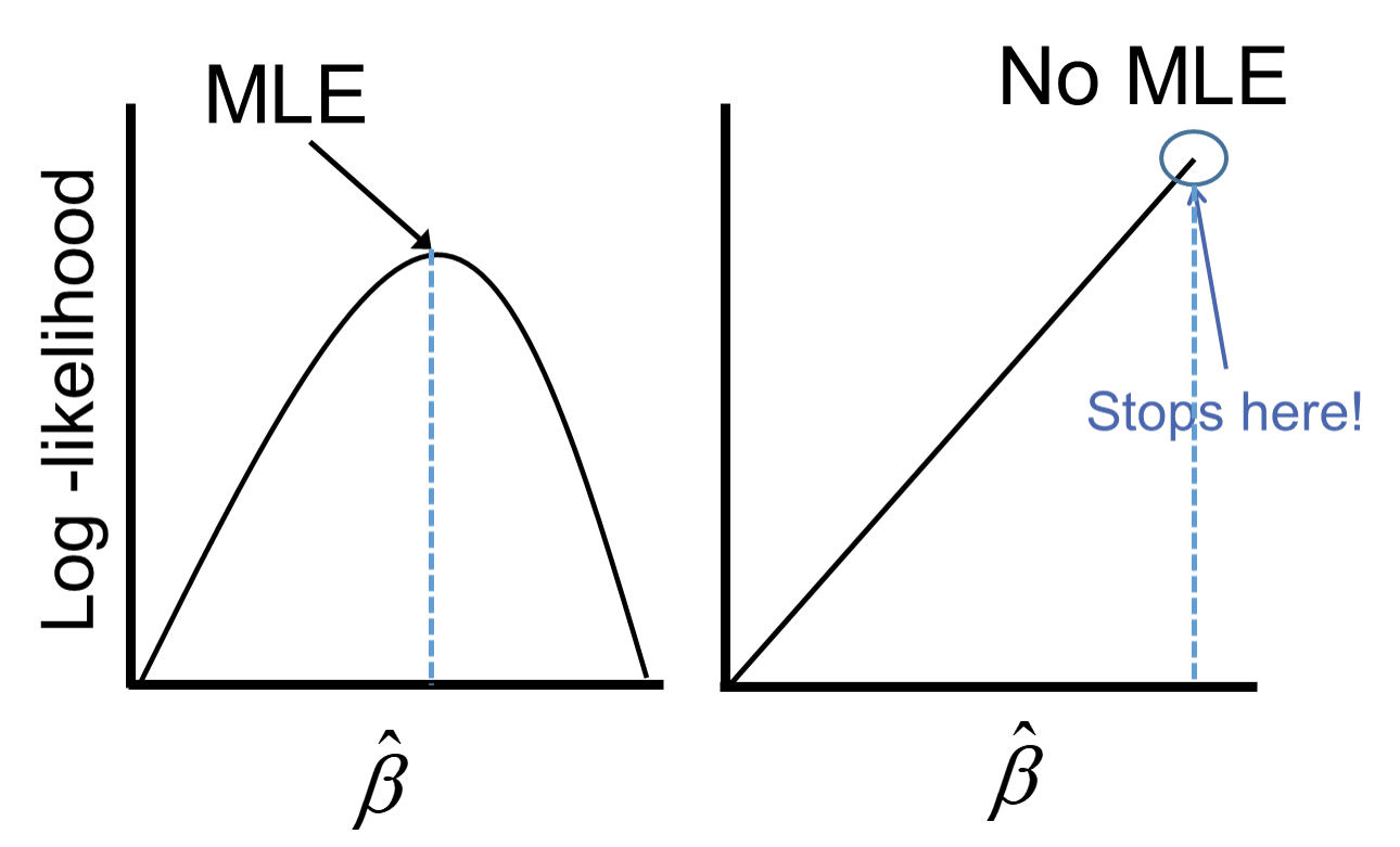
Remember that the logistic function is completely bounded within 0 and 1. Since these categories perfectly predict the target variable, we need a prediction of 0 or 1 for the probability which cannot be obtained in the logistic regression without infinitely positive (or negative) parameter estimates.

Let’s see if this is a problem in our data set (hint… it is!) and how to address this problem in our software!

Python
R

Ideally, we should explore all of our categorical variables before we ever model so separation issues shouldn’t be a surprise. Let’s examine our customer_service_calls variable using the crosstab function.

Code

pd.crosstab(index = train_u['churn'], columns = train_u['customer_service_calls'])

customer_service_calls   0   1   2   3   4  5  6  7
churn                                              
False                   27  38  23  13   1  1  1  0
True                    21  26  20  10  16  7  3  1

We can see that the category of 7 customer service calls predicts churn perfectly - 1 person churned while 0 did not. Every other category has at least one person who churned and one who didn’t so this is an example of quasi-complete separation.

In case you don’t explore your data ahead of time, you will notice interesting results in categories with separation issues. Let’s examine the parameter estimates for 7 customer service calls.

Code

from statsmodels.genmod.generalized_linear_model import GLM

predictors_q = train_u.drop(columns=['churn', 'weight'])
predictors_q['customer_service_calls'] = predictors_q['customer_service_calls'].astype(str)
predictors_q = pd.get_dummies(predictors_q, drop_first=True)
predictors_q = predictors_q.astype(float)

X_q = predictors_q
X_q = sm.add_constant(X_q)

y = train_u['churn']

weight_1 = 1
weight_0 = (2850/154) / (104/104)

train_u['weight'] = train_u.churn.replace({True: weight_1, False: weight_0}).astype(float)

model_w = sm.GLM(y, X_q, family = sm.families.Binomial(), freq_weights = train_u['weight'])
result_w = model_w.fit()
print(result_w.summary())

                 Generalized Linear Model Regression Results                  
==============================================================================
Dep. Variable:                  churn   No. Observations:                  208
Model:                            GLM   Df Residuals:                  2015.68
Model Family:                Binomial   Df Model:                           12
Link Function:                  Logit   Scale:                          1.0000
Method:                          IRLS   Log-Likelihood:                -313.68
Date:                Sat, 15 Nov 2025   Deviance:                       627.37
Time:                        10:55:00   Pearson chi2:                 2.94e+03
No. Iterations:                    19   Pseudo R-squ. (CS):             0.6048
Covariance Type:            nonrobust                                         
============================================================================================
                               coef    std err          z      P>|z|      [0.025      0.975]
--------------------------------------------------------------------------------------------
const                       -7.3488      0.765     -9.610      0.000      -8.848      -5.850
account_length               0.0019      0.003      0.654      0.513      -0.004       0.008
total_day_charge             0.1351      0.017      8.015      0.000       0.102       0.168
total_intl_calls            -0.1437      0.057     -2.502      0.012      -0.256      -0.031
international_plan_yes       2.0723      0.352      5.887      0.000       1.382       2.762
voice_mail_plan_yes         -0.5221      0.300     -1.738      0.082      -1.111       0.067
customer_service_calls_1    -0.1556      0.324     -0.480      0.631      -0.790       0.479
customer_service_calls_2    -0.2651      0.351     -0.755      0.450      -0.953       0.423
customer_service_calls_3     0.0375      0.418      0.090      0.928      -0.782       0.857
customer_service_calls_4     2.2857      0.488      4.684      0.000       1.329       3.242
customer_service_calls_5     2.3792      0.544      4.372      0.000       1.313       3.446
customer_service_calls_6     1.6549      0.742      2.231      0.026       0.201       3.109
customer_service_calls_7    24.9277   1.77e+04      0.001      0.999   -3.47e+04    3.48e+04
============================================================================================

Notice the category of 7 compared to the rest. It’s parameter estimates is rather high (remember that odds ratios are exponentiated parameter estimates so 20+ is REALLY large). That is a definite sign of convergence problems, especially since the p-value is close to 1!

Once possible solution to convergence problems in logistic regression is to perform exact logistic regression. This method is computationally more expensive and should really only be used if you need an estimate for the specific category that is causing the separation issues. Due to the computational expense we will use another solution.

A more common solution to separation concerns is to transform the categorical variable. Instead of having a category with separation issues, you can combine this category with another category to remove the separation concerns. Below we are creating a “4+” category that contains the categories of 4, 5, 6, and 7. This will remove the separation issues as you can see as we rerun the logistic regression.

Code

train_u['customer_service_calls_c'] = train_u['customer_service_calls']

train_u.loc[train_u['customer_service_calls'] >= 4, ['customer_service_calls_c']] = 4

pd.crosstab(index = train_u['churn'], columns = train_u['customer_service_calls_c'])

customer_service_calls_c   0   1   2   3   4
churn                                       
False                     27  38  23  13   3
True                      21  26  20  10  27

Code

predictors_q = train_u.drop(columns=['churn', 'weight', 'customer_service_calls'])
predictors_q['customer_service_calls_c'] = predictors_q['customer_service_calls_c'].astype(str)
predictors_q = pd.get_dummies(predictors_q, drop_first=True)
predictors_q = predictors_q.astype(float)

X_q = predictors_q
X_q = sm.add_constant(X_q)

y = train_u['churn']

weight_1 = 1
weight_0 = (2850/154) / (104/104)

train_u['weight'] = train_u.churn.replace({True: weight_1, False: weight_0}).astype(float)

<string>:2: FutureWarning: Downcasting behavior in `replace` is deprecated and will be removed in a future version. To retain the old behavior, explicitly call `result.infer_objects(copy=False)`. To opt-in to the future behavior, set `pd.set_option('future.no_silent_downcasting', True)`

Code

model_w = sm.GLM(y, X_q, family = sm.families.Binomial(), freq_weights = train_u['weight'])
result_w = model_w.fit()
print(result_w.summary())

                 Generalized Linear Model Regression Results                  
==============================================================================
Dep. Variable:                  churn   No. Observations:                  208
Model:                            GLM   Df Residuals:                  2018.68
Model Family:                Binomial   Df Model:                            9
Link Function:                  Logit   Scale:                          1.0000
Method:                          IRLS   Log-Likelihood:                -316.40
Date:                Sat, 15 Nov 2025   Deviance:                       632.80
Time:                        10:55:01   Pearson chi2:                 2.92e+03
No. Iterations:                     7   Pseudo R-squ. (CS):             0.5944
Covariance Type:            nonrobust                                         
==============================================================================================
                                 coef    std err          z      P>|z|      [0.025      0.975]
----------------------------------------------------------------------------------------------
const                         -7.2331      0.752     -9.621      0.000      -8.707      -5.760
account_length                 0.0009      0.003      0.330      0.741      -0.004       0.006
total_day_charge               0.1349      0.016      8.184      0.000       0.103       0.167
total_intl_calls              -0.1440      0.057     -2.518      0.012      -0.256      -0.032
international_plan_yes         2.0750      0.317      6.554      0.000       1.455       2.696
voice_mail_plan_yes           -0.5263      0.299     -1.759      0.079      -1.113       0.060
customer_service_calls_c_1    -0.1585      0.323     -0.490      0.624      -0.792       0.476
customer_service_calls_c_2    -0.2667      0.350     -0.761      0.447      -0.953       0.420
customer_service_calls_c_3     0.0439      0.417      0.105      0.916      -0.774       0.861
customer_service_calls_c_4     2.2660      0.373      6.076      0.000       1.535       2.997
==============================================================================================

Notice how we no longer have the large parameter estimates since we have corrected our convergence problems.

Code

table(train_u$customer_service_calls, train_u$churn)

   
    FALSE TRUE
  0    29   25
  1    34   25
  2    23   20
  3    15   12
  4     2   13
  5     1    4
  6     0    3
  7     0    2

We can see that the category of 6 customer service calls predicts churn perfectly - 3 person churned while 0 did not. Same for 7 customer service calls. Every other category has at least one person who churned and one who didn’t churn, so this is an example of quasi-complete separation.

In case you don’t explore your data ahead of time, you will notice interesting results in categories with separation issues. Let’s examine the parameter estimates for 6 and 7 customer service calls.

Code

logit.model.w <- glm(churn ~ factor(international_plan) +
                               factor(voice_mail_plan) +
                               total_day_charge +
                               factor(customer_service_calls),
                     data = train_u, family = binomial(link = "logit"),
                     weights = weight)
summary(logit.model.w)


Call:
glm(formula = churn ~ factor(international_plan) + factor(voice_mail_plan) + 
    total_day_charge + factor(customer_service_calls), family = binomial(link = "logit"), 
    data = train_u, weights = weight)

Coefficients:
                                  Estimate Std. Error z value Pr(>|z|)    
(Intercept)                      -10.14898    0.81614 -12.435  < 2e-16 ***
factor(international_plan)yes      3.29320    0.34765   9.473  < 2e-16 ***
factor(voice_mail_plan)yes        -0.99871    0.30330  -3.293 0.000992 ***
total_day_charge                   0.17916    0.01788  10.020  < 2e-16 ***
factor(customer_service_calls)1    0.49930    0.36184   1.380 0.167621    
factor(customer_service_calls)2    1.44557    0.40012   3.613 0.000303 ***
factor(customer_service_calls)3    1.22910    0.44653   2.753 0.005913 ** 
factor(customer_service_calls)4    3.61477    0.51999   6.952 3.61e-12 ***
factor(customer_service_calls)5    2.38244    0.69874   3.410 0.000651 ***
factor(customer_service_calls)6   22.86252  799.55896   0.029 0.977188    
factor(customer_service_calls)7   21.52806 1028.81098   0.021 0.983305    
---
Signif. codes:  0 '***' 0.001 '**' 0.01 '*' 0.05 '.' 0.1 ' ' 1

(Dispersion parameter for binomial family taken to be 1)

    Null deviance: 820.53  on 207  degrees of freedom
Residual deviance: 545.74  on 197  degrees of freedom
AIC: 571.92

Number of Fisher Scoring iterations: 14

Notice the category of 6 and 7 compared to the rest. Their parameter estimates are rather high (remember that odds ratios are exponentiated parameter estimates so 20+ is REALLY large). These are definite signs of convergence problems, especially considering the p-value for these is close to 1!

Once possible solution to convergence problems in logistic regression is to perform exact logistic regression. This method is computationally more expensive and should really only be used if you need an estimate for the specific category that is causing the separation issues. The logistf package in R can perform this analysis but is not shown here.

Code

train_u$customer_service_calls_c <- as.character(train_u$customer_service_calls)
train_u$customer_service_calls_c[which(train_u$customer_service_calls > 3)] <- "4+"

table(train_u$customer_service_calls_c, train_u$churn)

    
     FALSE TRUE
  0     29   25
  1     34   25
  2     23   20
  3     15   12
  4+     3   22

Code

logit.model.w <- glm(churn ~ factor(international_plan) +
                             factor(voice_mail_plan) +
                             total_day_charge +
                             factor(customer_service_calls_c),
                     data = train_u, family = binomial(link = "logit"),
                     weights = weight)
summary(logit.model.w)


Call:
glm(formula = churn ~ factor(international_plan) + factor(voice_mail_plan) + 
    total_day_charge + factor(customer_service_calls_c), family = binomial(link = "logit"), 
    data = train_u, weights = weight)

Coefficients:
                                   Estimate Std. Error z value Pr(>|z|)    
(Intercept)                        -9.18049    0.73431 -12.502  < 2e-16 ***
factor(international_plan)yes       3.08132    0.33255   9.266  < 2e-16 ***
factor(voice_mail_plan)yes         -1.14286    0.27819  -4.108 3.99e-05 ***
total_day_charge                    0.15726    0.01647   9.551  < 2e-16 ***
factor(customer_service_calls_c)1   0.44991    0.35419   1.270  0.20400    
factor(customer_service_calls_c)2   1.25333    0.38493   3.256  0.00113 ** 
factor(customer_service_calls_c)3   1.03757    0.43343   2.394  0.01667 *  
factor(customer_service_calls_c)4+  3.45947    0.42510   8.138 4.02e-16 ***
---
Signif. codes:  0 '***' 0.001 '**' 0.01 '*' 0.05 '.' 0.1 ' ' 1

(Dispersion parameter for binomial family taken to be 1)

    Null deviance: 820.53  on 207  degrees of freedom
Residual deviance: 580.00  on 200  degrees of freedom
AIC: 600.53

Number of Fisher Scoring iterations: 6

Notice how we no longer have the large parameter estimates since we have corrected our converge problems.

Ordinal variables are easy to combine categories because you can just combine separation categories with categories on either side. However, with nominal variables we typically combine the separation causing category with the category that has the relationship with the target variable that is the most similar. The following plot is an example of this:

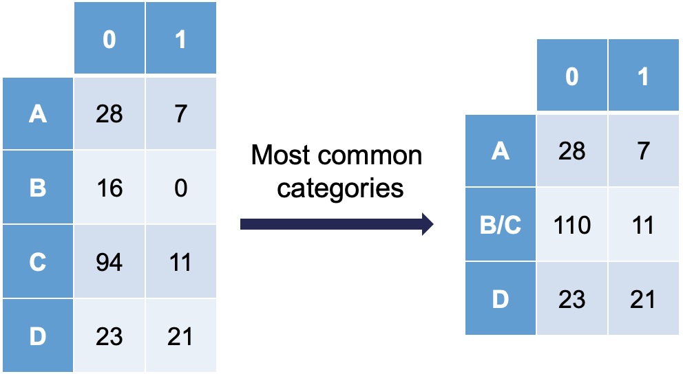
Notice how category C is most similar to category B (the problem category) in terms of its ratio of 0’s and 1’s. Formally, this method of combining categories is also called the Greenacre method.