Previously, we looked a binary logistic regression with only a couple of variables from our Ames housing data predicting bonus eligibility. However, to explore our data at scale we need to run many \(\chi^2\) tests like we learned from the Categorical Data Analysis section of the course deck to explore relationships between our categorical target variable and categorical predictors. We also need to evaluate relationships between the categorical target variable and continuous predictor variables. To evaluate those relationships we could run individual ANOVA calculations between the continuous and target variable or simple logistic regressions. The ANOVA calculations would be quicker due to not needing to optimize maximum likelihood estimation.
Let’s run these variable explorations in each software!
Before we can put the predictor variables in our functions for automated screening we need to convert our categorical predictor variables into dummy coded variables. Essentially, we need to one-hot encode our variables to make each category have a corresponding binary flag variable. Using the get_dummies function from Pandas we can do this easily. First, we must remove the target variable from our training data with the drop function. Just to make sure that all variables are of the same type, after converting the variables to binary flags we use the astype(float) function on all our predictor variables. Lastly, we call the predictor variables dataframe X and our target variable y.
Once our data is in this format we can use the SelectKBest,chi2, and f_classif functions from the popular sci-kit learn package, specifically sklearn.feature_selection. Inside SelectKBest we will use the f_classif and chi2 functions as our scoring functions for continuous and categorical predictors respectively.
First we will explore the categorical predictor variables. However, since we have already dummy coded all of our caetgorical variables, to isolate just the categorical variables we can isolate the variables with only two unique values using the unique function inside of a for loop.
Once we isolate the categorical variables into their own X_cat object we can use the SelectKBest function with the score_func = chi2 option. The k = 'all' option doesn’t eliminate any variables, but instead calculates the p-value for each variable. That way we can be the ones to decide which variables we want to keep. We then input our X_cat and y objects into the fit function on the SelectKBest object. From there we just save the column names (columns), the test statistics (scores_), and p-values (pvalues_) into a single dataframe. From here we can remove the variables with a p-value above our 0.009 cut-off by isolating the specific variables that meet that requirement.
Code
from sklearn.feature_selection import SelectKBest, chi2, f_classif# Separate categorical (dummy) vs. continuous featurescategorical_features = [col for col in X.columns if X[col].nunique() ==2]continuous_features = [col for col in X.columns if X[col].nunique() >2]X_cat = X[categorical_features]X_cont = X[continuous_features]# Fit SelectKBest for Categorical Variablesselector = SelectKBest(score_func=chi2, k='all') # 'all' keeps all features for scoringselector.fit(X_cat, y)
SelectKBest(k='all', score_func=<function chi2 at 0x32a21a7a0>)
In a Jupyter environment, please rerun this cell to show the HTML representation or trust the notebook. On GitHub, the HTML representation is unable to render, please try loading this page with nbviewer.org.
Parameters
score_func
<function chi2 at 0x32a21a7a0>
k
'all'
Code
# Create a DataFrame with feature names, Chi2-scores, and p-valuesscores_cat_df = pd.DataFrame({'Feature': X_cat.columns,'Chi2_score': selector.scores_,'p_value': selector.pvalues_})# Filter for features with p-value < 0.009selected_cat_features = scores_cat_df[scores_cat_df['p_value'] <0.009]['Feature']
Next we will explore the continuous predictor variables we obtained from the previous code.
Once we isolate the continuous variables into their own X_cont object we can use the SelectKBest function with the score_func = f_classif option. The k = 'all' option doesn’t eliminate any variables, but instead calculates the p-value for each variable. That way we can be the ones to decide which variables we want to keep. We then input our X_cont and y objects into the fit function on the SelectKBest object. From there we just save the column names (columns), the test statistics (scores_), and p-values (pvalues_) into a single dataframe. From here we can remove the variables with a p-value above our 0.009 cut-off by isolating the specific variables that meet that requirement. We then select only those variables from our original X object to get our reduced variable list called X_reduced.
Code
# Fit SelectKBest for Continous Variablesselector = SelectKBest(score_func=f_classif, k='all') # 'all' keeps all features for scoringselector.fit(X_cont, y)
SelectKBest(k='all')
In a Jupyter environment, please rerun this cell to show the HTML representation or trust the notebook. On GitHub, the HTML representation is unable to render, please try loading this page with nbviewer.org.
Parameters
score_func
<function f_c...t 0x32a21a5c0>
k
'all'
Code
# Create a DataFrame with feature names, F-scores, and p-valuesscores_cont_df = pd.DataFrame({'Feature': X_cont.columns,'F_score': selector.scores_,'p_value': selector.pvalues_})# Filter for features with p-value < 0.009selected_cont_features = scores_cont_df[scores_cont_df['p_value'] <0.009]['Feature']# Create a new DataFrame with only those selected columnsX_reduced = X[selected_cat_features.tolist() + selected_cont_features.tolist()]X_reduced.head()
Before we can put the predictor variables in our functions for automated screening we need to convert our categorical variables into dummy coded variables. Essentially, we need to one-hot encode our variables to make each category have a corresponding binary flag variable. Using the model.matrix function we can do this easily. First, we must remove the target variable from our training data with the select function. Lastly, we call the predictor variables dataframe X and our target variable y.
Code
library(broom)library(dplyr)train$bonus <-as.integer(train$SalePrice >175000)predictors <- train %>%select(-SalePrice, -bonus)# Create dummy variables (drop first level to avoid multicollinearity)predictors_dummies <-model.matrix(~ . -1, data = predictors)predictors_dummies <-as.data.frame(predictors_dummies)predictors_dummies <- predictors_dummies %>%select(-GarageTypeMissing, -GarageQualMissing, -GarageCondMissing)# Final features and targetX <- predictors_dummiesy <- train$bonus
Once our data is in this format we can use the lapply function. Inside lapply we will use the aov and chisq.test functions as our scoring functions for continuous and categorical predictors respectively.
First we will explore the categorical predictor variables. However, since we have already dummy coded all of our categorical variables, to isolate just the categorical variables we can isolate the variables with only two unique values using the length and unique functions inside of an sapply function.
Once our data is in this format we can use the lapply function and input our own function where we calculate the individual \(\chi^2\) tests. We will create our own function where we calculate individual \(\chi^2\) tests with the chisq.test function. From those individual tests we use the p.value and statistic elements to extract the p-value and test statistic information. This approach doesn’t eliminate any variables, but instead calculates the p-value for each variable. That way we can be the ones to decide which variables we want to keep. From here we can remove the variables with a p-value above our 0.009 cut-off by isolating the specific variables that meet that requirement.
Code
# Separate categorical and continuous featurescategorical_features <-names(X)[sapply(X, function(col) length(unique(col)) ==2)]continuous_features <-names(X)[sapply(X, function(col) length(unique(col)) >2)]X_cat <- X[, categorical_features, drop =FALSE]X_cont <- X[, continuous_features, drop =FALSE]# ---- Chi-squared test for categorical features ----chi2_results <-lapply(names(X_cat), function(col) { tbl <-table(X_cat[[col]], y) test <-suppressWarnings(chisq.test(tbl))data.frame(Feature = col,Chi2_score = test$statistic,p_value = test$p.value )})chi2_df <-do.call(rbind, chi2_results)# Select features with p-value < 0.009selected_cat_features <- chi2_df %>%filter(p_value <0.009) %>%pull(Feature)
Next we will explore the continuous predictor variables we obtained from the previous code.
Once we isolate the continuous variables into their own X_cont object we can use the lapply function with the aov function within it. Similar to above, we will create our own function where we calculate individual ANOVA F tests with the aov function. From those individual ANOVA’s we use the summary function to extract the p-value and test statistic information. This approach doesn’t eliminate any variables, but instead calculates the p-value for each variable. That way we can be the ones to decide which variables we want to keep. From here we can remove the variables with a p-value above our 0.009 cut-off by isolating the specific variables that meet that requirement. We then select only those variables from our original X object to get our reduced variable list called X_reduced.
Code
# ---- ANOVA F-test for continuous features ----anova_results <-lapply(names(X_cont), function(col) { model <-aov(X_cont[[col]] ~as.factor(y)) test <-summary(model)[[1]]data.frame(Feature = col,F_score = test$`F value`[1],p_value = test$`Pr(>F)`[1] )})anova_df <-do.call(rbind, anova_results)# Select features with p-value < 0.009selected_cont_features <- anova_df %>%filter(p_value <0.009) %>%pull(Feature)# ---- Combine selected features ----selected_features <-c(selected_cat_features, selected_cont_features)# Create reduced feature setX_reduced <- X[, selected_features, drop =FALSE]# View first few rowshead(X_reduced, n =5)
In the previous section of the code deck we talked about looking at quasi-complete separation. To make sure that our data doesn’t have variables that have quasi complete separation concerns, we can write a function to check our data and then combine those categories with reference categories for the variable.
In Python it is a simple task to write a function. We will call our function check_quasi_complete_separation with two inputs - our predictor variables and our target variable. Inside this function we are calculating the crosstab function from pandas and looking for any cells with 0’s with the any function. If there are any cells with values of 0’s which would lead to quasi-complete separation we will print them out.
Code
def check_quasi_complete_separation(X, y):""" Checks each categorical predictor in X for quasi-complete separation with respect to binary target y. Parameters: - X: pd.DataFrame of predictors (categorical variables) - y: pd.Series of binary target variable (e.g., 0/1 or True/False) Returns: - List of variable names that exhibit quasi-complete separation """ problematic_vars = []for col in X.columns: ct = pd.crosstab(X[col], y)# Check if any category (row) has a zero in any outcome classif (ct ==0).any(axis=1).any():print(f"⚠️ Quasi-complete separation detected in '{col}'")print(ct)print() problematic_vars.append(col)return problematic_vars
Let’s now put our actual data in the function. We only want to do this check on categorical predictor variables.
Looks like we have a couple of variables with quasi-complete separation. Let’s remove these variables from our dataset before building our model.
Code
X_reduced = X_reduced.drop(problem_vars, axis =1)
In R it is a simple task to write a function. We will call our function check_quasi_complete_separation with two inputs - our predictor variables and our target variable. Inside this function we are calculating the table function and looking for any cells with 0’s with the any and apply functions. If there are any cells with values of 0’s which would lead to quasi-complete separation we will print them out.
Code
check_quasi_complete_separation <-function(X, y) {# X: data.frame of categorical predictors# y: binary target (factor or 0/1 vector) problematic_vars <-c()for (colname innames(X)) { ct <-table(X[[colname]], y)# Check if any row has a zero in any column (i.e., any category lacks one class) has_zero <-apply(ct, 1, function(row) any(row ==0))if (any(has_zero)) {cat("⚠️ Quasi-complete separation detected in '", colname, "'\n", sep ="")print(ct)cat("\n") problematic_vars <-c(problematic_vars, colname) } }return(problematic_vars)}
Let’s now put our actual data in the function. We only want to do this check on categorical predictor variables.
Which variables should you drop from your model? This is a common question for all modeling, including logistic regression. In this section we will cover a popular variable selection technique - stepwise regression. This isn’t the only possible technique, but will be the primary focus here.
Stepwise regression techniques involve the three common methods:
Forward Selection
Backward Selection
Stepwise Selection
These techniques add or remove (depending on the technique) one variable at a time from your regression model to try and “improve” the model. There are a variety of different selection criteria to use to add or remove variables from a logistic regression which will be covered in more detail in the model assessment part of the code deck.
The specific details of each of these is covered in full in the Model Building portion of this code deck. Let’s revisit what stepwise selection is doing.
Stepwise Selection
Let’s revisit the stepwise selection approach with cross-validation specifically.
Stepwise Variable Selection with CV
In first step of the stepwise selection process, we create models such that each model has exactly one predictor variable and calculate a model metric for each model. However, we do this across each cross-validation training set. For 10-fold cross-validation, that would be 10 separate first steps that create models with only one variable. Next, we average the model metric across all cross-validation training sets to see which is the best variable. For example, the 5th variable is now the best on average across all of the cross-validation datasets based on our model metric, not just the training set overall.
This same process is repeated across all of the steps until a final model is selected where adding any further variables does not improve the model based on the cross-validation model metrics. Remember, the difference between forward and stepwise selection is that we are also evaluating each variable added to the model at each step to see if deleting that variable improves the model metric.
To gain the needed functionality for cross-validation recursive feature addition or subtraction, we need to use the mlxtend package on top of scikit-learn. Specifically, we will use the SequentialFeatureSelector function from mlxtend.feature_selection. We will need to create our logistic regression object with the LogisticRegression function, not the statsmodels.api version with the Logit function. We need the penalty = None option to perform traditional logistic regression with no additional penalties (discussed in the Regularization section of the code deck). This object will be an input to our SFS function. We also need an additional step to improve the speed of the feature selection - scaling the data. This will help improve the speed of the maximum llikelihood optimization. To do this we will use the StandardScaler function from the sklearn.processing package. We will take the reduced data frame of the predictors, X_reduced, and input it into the StandardScaler object with the fit_transform function. This function unfortunately doesn’t produce a data frame output so we have to turn this into a data frame with the pandasDataFrame function with the columns option to define the same columns as we had with the reduced dataset.
Now we can define our SFS function. In the k_features option we can put any integer value to set a certain number of features, the "best" option to pick the number of features that provides the best value of the model metric, or the "parsimonious" option to pick the number of features within one standard error of the true best model to try and make the model simpler. The forward = True option makes the function perform forward selection. The floating = True option means that once a variable is added it is evaluated at each step to be dropped out of the model - stepwise selection. The scoring option allows you to select your model metric. The options for a binary target variable are the accuracy, precision, recall, F1 score, area under the ROC curve (roc_auc), negative log loss, and negative Brier score. These will be covered in much further detail in the next section of the code deck on Model Assessment. The reason the last two are negative is that the function tries to maximize the optimization function. The cv option allows you to pick the number of cross-validation folds. Lastly, we just use the fit function with our predictor variables and target variable to fit the model. The variables are then printed below.
Code
from mlxtend.feature_selection import SequentialFeatureSelector as SFSfrom sklearn.linear_model import LogisticRegressionfrom sklearn.preprocessing import StandardScalerscaler = StandardScaler()X_scaled = scaler.fit_transform(X_reduced)X_scaled_df = pd.DataFrame(X_scaled, columns = X_reduced.columns)logr = LogisticRegression(max_iter =1000, solver ='newton-cg', penalty =None) # Backward selection to find best subset of featuressfs = SFS(logr, k_features ="best", forward =True, floating =True, scoring ='roc_auc', cv =10)sfs = sfs.fit(X_scaled_df, y)# Get selected feature namesselected_features =list(sfs.k_feature_names_)print("Selected features:", selected_features)
Now we have variables determined by stepwise selection with cross-validation.
To gain the needed functionality for cross-validation recursive feature addition or subtraction, we need to use the caret package. Specifically, we will use the train function from caret package along with the MASS package. The caret function can not handle our target variable and predictor variables being in separate objects. Therefore, we first use cbind to combine the target variable as a column to the predictor variables dataframe. Now we can use the new dataframe to put into caret with the typical formula structure we have used previously. We also need to make our target variable a factor object using the factor function for the package to fit the correct model.
The method = "glmStepAIC" option uses the MASS package and its stepwise selection capabilities. You can think of caret as more of a wrapper function that puts a cross-validation spin on other functions.
The glmStepAIC function that does recursive feature elimination such as stepwise selection uses likelihood based metrics to selection variables. We will use two of the most common ones: AIC and BIC (can also be referred to as SBC).
The AIC, or Akaike Information Criterion, was developed by statistician Hirotugu Akaike in the 1970’s and is defined by:
\[
AIC = n \log(\frac{SSE}{n}) + 2(p + 1)
\]
In this case, the \(SSE\) is the sum of squared error from the model and \(2(p+1)\) is the “penalty”, where \(p\) is the number of variables in the model. A smaller AIC indicates a better model.
BIC, also known as the Bayesian Information Criterion (also called SBC or Schwarz Bayesian Information) was first developed by Gideon E. Schwarz, also back in the 1970’s and is defined by:
\[
BIC = n \log(\frac{SSE}{n}) + (p+1)\log (n)
\]
In this case, “Likelihood” is the likelihood of the data and \((p+1)\log(n)\) is the “penalty”, where \(p\) is the number of variables in the model and \(n\) is the sample size. A smaller BIC indicates a better model. This is how variables are selected at each step in the stepwise selection.
However, the metric option allows you to select your model metric across cross-validation training sets to pick the best one. The options for a binary target variable are controlled with the summaryFuction option in the trainControl function. The trControl = trainControl(method = 'cv', number = 10)) option allows you to pick the number of cross-validation folds. That summary function allows different evaluation metrics. We can pick the F1 score, precision, recall, area under the ROC curve (AUC), and area under the precision-recall curve. Using other optoins in the summaryFunction provides even more possible metrics. We also have to specify the fmaily = "binomial option to build a logistic regression and the direction = "both" option to specify we want stepwise selection. The results object will display our final performance metric and the summary function will show a summary of the final model built.
Now we have variables determined by stepwise selection with cross-validation.
Backward Selection
Let’s also revisit the backward selection approach with cross-validation.
Backward Variable Elimination with CV
In first step of the backward selection process, we create models such that each model has exactly one predictor variable removed from it and calculate a model metric for each model. However, we do this across each cross-validation training set. For 10-fold cross-validation, that would be 10 separate first steps that create models removing only one variable. Next, we average the model metric across all training sets to see which is the worst variable. For example, the second variable is now the worst on average across all of the cross-validation datasets based on our model metric, not just the training set overall.
This same process is repeated across all of the steps until a final model is selected where removing any further variables does not improve the model based on the cross-validation model metrics.
To gain the needed functionality for cross-validation recursive feature addition or subtraction, we need to use the mlxtend package on top of scikit-learn. Specifically, we will use the SequentialFeatureSelector function from mlxtend.feature_selection. We will need to create our logistic regression object with the LogisticRegression function, not the statsmodels.api version with the Logit function. We need the penalty = None option to perform traditional logistic regression with no additional penalties (discussed in the Regularization section of the code deck). This object will be an input to our SFS function. We also need an additional step to improve the speed of the feature selection - scaling the data. This will help improve the speed of the maximum llikelihood optimization. To do this we will use the StandardScaler function from the sklearn.processing package. We will take the reduced data frame of the predictors, X_reduced, and input it into the StandardScaler object with the fit_transform function. This function unfortunately doesn’t produce a data frame output so we have to turn this into a data frame with the pandasDataFrame function with the columns option to define the same columns as we had with the reduced dataset.
Now we can define our SFS function. In the k_features option we can put any integer value to set a certain number of features, the "best" option to pick the number of features that provides the best value of the model metric, or the "parsimonious" option to pick the number of features within one standard error of the true best model to try and make the model simpler. The forward = False and floating = False options makes the function perform backward selection. The scoring option allows you to select your model metric. The options for a binary target variable are the accuracy, precision, recall, F1 score, area under the ROC curve (roc_auc), negative log loss, and negative Brier score. These will be covered in much further detail in the next section of the code deck on Model Assessment. The reason the last two are negative is that the function tries to maximize the optimization function. The cv option allows you to pick the number of cross-validation folds. Lastly, we just use the fit function with our predictor variables and target variable to fit the model. The variables are then printed below.
Code
from mlxtend.feature_selection import SequentialFeatureSelector as SFSfrom sklearn.linear_model import LogisticRegressionfrom sklearn.preprocessing import StandardScalerscaler = StandardScaler()X_scaled = scaler.fit_transform(X_reduced)X_scaled_df = pd.DataFrame(X_scaled, columns = X_reduced.columns)logr = LogisticRegression(max_iter =1000, solver ='newton-cg', penalty =None) # Backward selection to find best subset of featuressfs = SFS(logr, k_features ="best", forward =False, floating =False, scoring ='roc_auc', cv =10)sfs = sfs.fit(X_scaled_df, y)# Get selected feature namesselected_features =list(sfs.k_feature_names_)print("Selected features:", selected_features)
Now we have variables determined by backward selection using cross-validation. Let’s see this final model using its variables in the traditional Logit function from statsmodels.
Most of the variables are similar to the ones we had from stepwise selection with some slight variations.
To gain the needed functionality for cross-validation recursive feature addition or subtraction, we need to use the caret package. Specifically, we will use the train function from caret package along with the MASS package. The caret function can not handle our target variable and predictor variables being in separate objects. Therefore, we first use cbind to combine the target variable as a column to the predictor variables dataframe. Now we can use the new dataframe to put into caret with the typical formula structure we have used previously. We also need to make our target variable a factor object using the factor function for the package to fit the correct model.
The method = "glmStepAIC" option uses the MASS package and its backward selection capabilities. You can think of caret as more of a wrapper function that puts a cross-validation spin on other functions. The glmStepAIC function that does recursive feature elimination such as backward selection uses likelihood based metrics to selection variables just like we discussed with the stepwise selection above.
However, the metric option allows you to select your model metric across cross-validation training sets to pick the best one. The options for a binary target variable are controlled with the summaryFuction option in the trainControl function. The trControl = trainControl(method = 'cv', number = 10)) option allows you to pick the number of cross-validation folds. That summary function allows different evaluation metrics. We can pick the F1 score, precision, recall, area under the ROC curve (AUC), and area under the precision-recall curve. Using other optoins in the summaryFunction provides even more possible metrics. We also have to specify the fmaily = "binomial option to build a logistic regression and the direction = "backward" option to specify we want backward selection. The results object will display our final performance metric and the summary function will show a summary of the final model built.
Now we have variables determined by backward selection using cross-validation. Most of the variables are similar to the ones we had from stepwise selection with some slight variations.
Forward Selection with Interactions
Here we will work through forward selection. In forward selection, the initial model is empty (contains no variables, only the intercept). Each variable is then tried to see how much it improves a model based on a model metric. The most important variable (based on that metric) is then added to the model. Then the remaining variables are again tested and the next most impactful variable (based on the same model metric) is added to the model. This process repeats until either no more variables are available to add to the model based on the metric. This approach is the same as stepwise selection without the additional check at each step for possible removal.
Forward selection is the least used technique because stepwise selection does the same as forward selection with the added benefit of dropping insignificant variables. The main use for forward selection is to test higher order terms and interactions in models. You can start with your model determined from either stepwise or backward selection and then try to add only interactions between variables from there.
The code for this is not shown here, but it is a simple change to the code above to perform this approach.
Calibration Curves
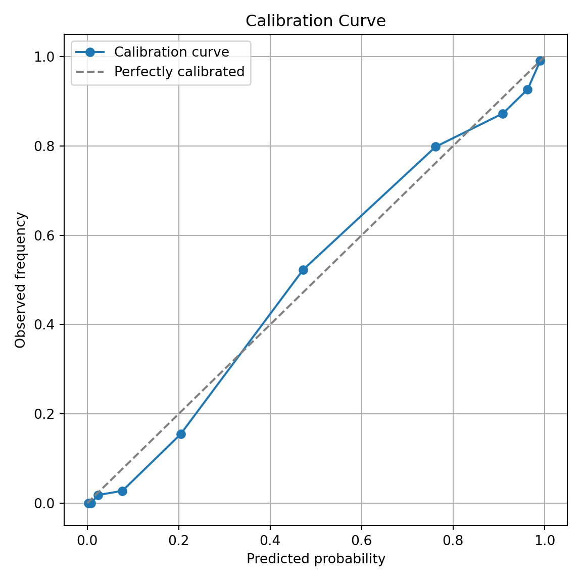
Another evaluation/diagnostic for logistic regression is the calibration curve. The calibration curve is a goodness-of-fit measure for logistic regression. Calibration measures how well predicted probabilities agree with actual frequency counts of outcomes (estimated linearly across the data set). These curves can help detect if predictions are consistently too high or low in your model.
If the curve is above the diagonal line, this indicates the model is predicting lower probabilities than actually observed. The opposite is true if the curve is below the diagonal line.
This is best used on larger samples since we are calculating the observed proportion of events in the data. In smaller samples this relationship is extrapolated out from the center and may not as accurately reflect the truth.
To build a calibration curve in Python we can use the calibration_curve function inside of the sklearn.calibration package. The input to this function are the target variable, bonus, and our predicted probabilities from our data. To get these predicted values we can use the predict function on our model object called result. The inputs for this predict function are a dataset we want to score. We will calculate the predicted probabilities of our training dataset. The model we are using comes from the backward selection from above. The other options in the calibration_curve function in Python is how many bins you want to compute the goodness-of-fit (here we use 10) and the strategy for this calculation. We will use the strategy = 'quantile' option. This option breaks our data into 10 groups of equal sizes of observations instead of just splitting the probabilities into groups of 0-0.1, 0.1-0.2, etc.
The calibration_curve function produces two outputs - the fraction of positives in each bin (the true probability) and the average predicted probability of each bin. These should be close to each other for the model to be well calibrated. The rest of the code is just used to plot this calibration curve.
Since the calibration curve line is consistently along the straight line, we do not notice any significant number of over or under predictions.
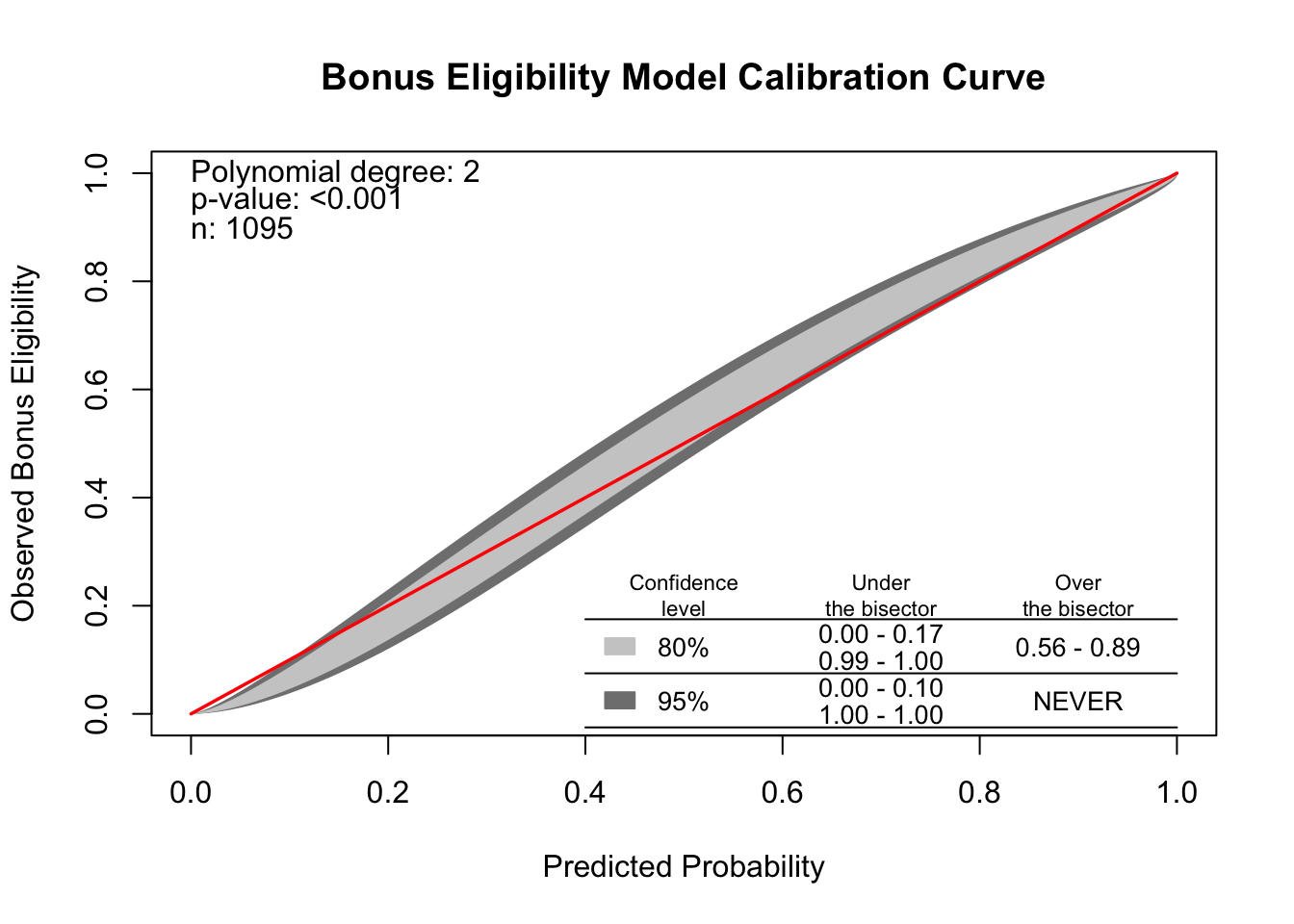
R produces a calibration curve using the givitiCalibrationBelt function. The inputs to this function are o = and e =. These are the observed target and expected (predicted) target respectively. To get these predicted values we can use the predict function on our model object called back_model. We will calculate the predicted probabilities of our training dataset. The model we are using comes from the backward selection from above. We place our actual target variable in the o = option and the predictions from our logistic regression model in the e = option. Since the model is being compared to training data the devel = internal option is specified. The maxDeg = option sets the maximum degree being tested for the curve.
Code
library(givitiR)cali.curve <-givitiCalibrationBelt(o = train$bonus,e =predict(back_model, type ="prob")[, "yes"],devel ="internal",maxDeg =5)plot(cali.curve, main ="Bonus Eligibility Model Calibration Curve",xlab ="Predicted Probability",ylab ="Observed Bonus Eligibility")
$m
[1] 2

$p.value
[1] 5.706546e-13
Since the diagonal line is contained in the confidence interval for our calibration curve, we do not notice any significant number of over or under predictions.
Diagnostic Plots
Linear regression models contain residuals with properties that are very useful for model diagnostics. However, what is a residual in a logistic regression model? Since we don’t have actual probabilities to compare our predicted probabilities against, residuals are not as clearly defined. Instead we have pseudo “residuals” in logistic regression that we can explore further. Two examples of this are deviance residuals and Pearson residuals.
Deviance is a measure of how far a fitted model is from the fully saturated model. The fully saturated model is a model that predicts our data perfectly by essentially overfitting to it - a variable for each unique combination of inputs. This makes this model impractical for use, but good for comparison. The deviance is essentially our “error” from this “perfect” model. Logistic regression minimizes the sum of the squared deviances. Deviance residuals tell us how much each observation reduces the deviance.
Pearson residuals on the other hand tell us how much each observation changes the Pearson Chi-squared test for the overall model.
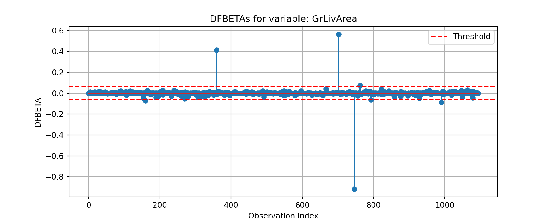
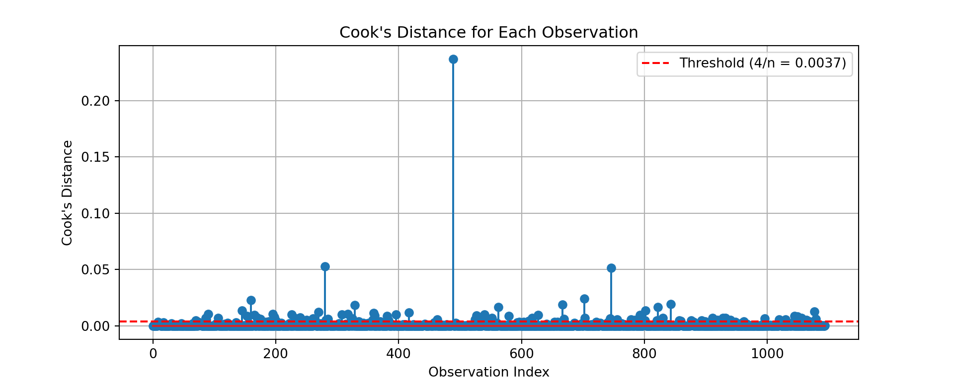
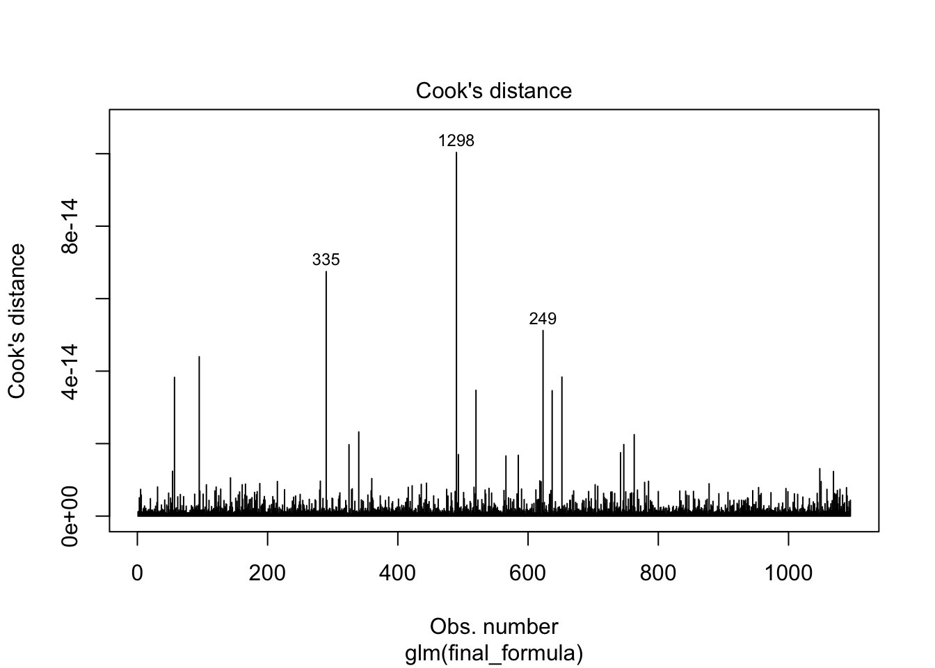
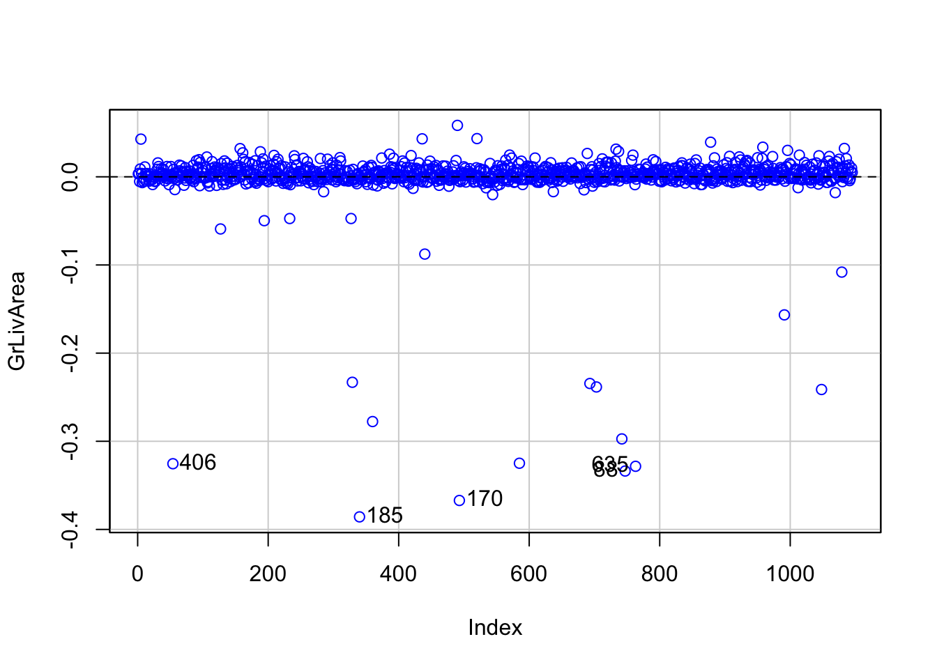
Other forms of measuring an observation’s influence on the logistic regression model are DFBetas and Cook’s D. Similar to their interpretation in linear regression, these two calculations tell us how each observation changes the estimation of each parameter individually (DFBeta) or how each observation changes the estimation of all the parameters holistically (Cook’s D).
Let’s see how to get all of these from each software!
Python has some wonderful diagnostics plots to show us these residuals. Python also produces a list of these measures of influence as well as many more with the get_influence function. Below only the first 5 observations are shown using the head function, but this is calculated for each of the observations.
The output above has all of the needed information. We can get both Cook’s D and DFBeta’s from the above summary as well as many other metrics. The following code just takes the Cook’s D values and DFBeta values and plots them. Only one of the DFBetas plots is actually shown.
cooks_d = influence.cooks_distance[0]n =len(cooks_d)threshold =4/ nplt.figure(figsize=(10, 4))plt.stem(cooks_d)plt.axhline(y=threshold, color='red', linestyle='--', label=f'Threshold (4/n = {threshold:.4f})')plt.title("Cook's Distance for Each Observation")plt.xlabel('Observation Index')plt.ylabel("Cook's Distance")plt.legend()plt.grid(True)plt.show()
R has some wonderful diagnostics plots to show us these residuals. R also produces a list of these measures of influence as well as many more with the influence.measures function. Below only the first 6 observations are shown using the head function, but this is calculated for each of the observations. The 4th plot in the plot function on the logistic regression model object is the Cook’s D plot as shown below. The dfbetasPlots function produces the DFBetas plots, but only one is shown here.
---title: "Subset Selection"format: html: code-fold: show code-tools: trueengine: knitreditor: visual---```{r}#| include: false#| warning: false#| error: false#| message: falselibrary(reticulate)reticulate::use_condaenv("wfu_fall_ml", required =TRUE)``````{python}#| include: false#| warning: false#| error: false#| message: falsefrom sklearn.datasets import fetch_openmlimport pandas as pdfrom sklearn.feature_selection import SelectKBest, f_classifimport numpy as npimport matplotlib.pyplot as plt# Load Ames Housing datadata = fetch_openml(name="house_prices", as_frame=True)ames = data.frame# Remove Business Logic Variablesames = ames.drop(['Id', 'MSSubClass','Functional','MSZoning','Neighborhood', 'LandSlope','Condition2','OverallCond','RoofStyle','RoofMatl','Exterior1st','Exterior2nd','MasVnrType','MasVnrArea','ExterCond','BsmtCond','BsmtExposure','BsmtFinType1','BsmtFinSF1','BsmtFinType2','BsmtFinSF2','BsmtUnfSF','Electrical','LowQualFinSF','BsmtFullBath','BsmtHalfBath','KitchenAbvGr','GarageFinish','SaleType','SaleCondition'], axis=1)# Remove Missingness Variablesames = ames.drop(['PoolQC', 'MiscFeature','Alley', 'Fence'], axis=1)# Impute Missingness for Categorical Variablescat_cols = ames.select_dtypes(include=['object', 'category']).columnsames[cat_cols] = ames[cat_cols].fillna('Missing')# Remove Low Variability Variablesames = ames.drop(['Street', 'Utilities','Heating'], axis=1)# Train / Test Splitfrom sklearn.model_selection import train_test_splittrain, test = train_test_split(ames, test_size =0.25, random_state =1234)# Impute Missing for Continuous Variablesnum_cols = train.select_dtypes(include='number').columnsfor col in num_cols:if train[col].isnull().any():# Create missing flag column train[f'{col}_was_missing'] = train[col].isnull().astype(int)# Impute with median median = train[col].median() train[col] = train[col].fillna(median)``````{r}#| include: false#| warning: false#| error: false#| message: falsetrain = py$traintest = py$test```# Preparing the DataPreviously, we looked a binary logistic regression with only a couple of variables from our Ames housing data predicting bonus eligibility. However, to explore our data at scale we need to run many $\chi^2$ tests like we learned from the Categorical Data Analysis section of the course deck to explore relationships between our categorical target variable and categorical predictors. We also need to evaluate relationships between the categorical target variable and continuous predictor variables. To evaluate those relationships we could run individual ANOVA calculations between the continuous and target variable or simple logistic regressions. The ANOVA calculations would be quicker due to not needing to optimize maximum likelihood estimation.Let's run these variable explorations in each software!::: {.panel-tabset .nav-pills}## PythonBefore we can put the predictor variables in our functions for automated screening we need to convert our categorical predictor variables into dummy coded variables. Essentially, we need to one-hot encode our variables to make each category have a corresponding binary flag variable. Using the `get_dummies` function from Pandas we can do this easily. First, we must remove the target variable from our training data with the `drop` function. Just to make sure that all variables are of the same type, after converting the variables to binary flags we use the `astype(float)` function on all our predictor variables. Lastly, we call the predictor variables dataframe `X` and our target variable `y`.```{python}#| warning: false#| error: false#| message: falsetrain['bonus'] = (train['SalePrice'] >175000).astype(int)predictors = train.drop(columns=['SalePrice', 'bonus'])predictors = pd.get_dummies(predictors, drop_first=True)predictors = predictors.astype(float)predictors = predictors.drop(['GarageType_Missing', 'GarageQual_Missing','GarageCond_Missing'], axis=1)X = predictorsy = train['bonus']```Once our data is in this format we can use the `SelectKBest`,`chi2`, and `f_classif` functions from the popular sci-kit learn package, specifically `sklearn.feature_selection`. Inside `SelectKBest` we will use the `f_classif` and `chi2` functions as our scoring functions for continuous and categorical predictors respectively.First we will explore the categorical predictor variables. However, since we have already dummy coded all of our caetgorical variables, to isolate just the categorical variables we can isolate the variables with only two unique values using the `unique` function inside of a `for` loop.Once we isolate the categorical variables into their own `X_cat` object we can use the `SelectKBest` function with the `score_func = chi2` option. The `k = 'all'` option doesn't eliminate any variables, but instead calculates the p-value for each variable. That way we can be the ones to decide which variables we want to keep. We then input our `X_cat` and `y` objects into the `fit` function on the `SelectKBest` object. From there we just save the column names (`columns`), the test statistics (`scores_`), and p-values (`pvalues_`) into a single dataframe. From here we can remove the variables with a p-value above our 0.009 cut-off by isolating the specific variables that meet that requirement.```{python}#| warning: false#| error: false#| message: falsefrom sklearn.feature_selection import SelectKBest, chi2, f_classif# Separate categorical (dummy) vs. continuous featurescategorical_features = [col for col in X.columns if X[col].nunique() ==2]continuous_features = [col for col in X.columns if X[col].nunique() >2]X_cat = X[categorical_features]X_cont = X[continuous_features]# Fit SelectKBest for Categorical Variablesselector = SelectKBest(score_func=chi2, k='all') # 'all' keeps all features for scoringselector.fit(X_cat, y)# Create a DataFrame with feature names, Chi2-scores, and p-valuesscores_cat_df = pd.DataFrame({'Feature': X_cat.columns,'Chi2_score': selector.scores_,'p_value': selector.pvalues_})# Filter for features with p-value < 0.009selected_cat_features = scores_cat_df[scores_cat_df['p_value'] <0.009]['Feature']```Next we will explore the continuous predictor variables we obtained from the previous code.Once we isolate the continuous variables into their own `X_cont` object we can use the `SelectKBest` function with the `score_func = f_classif` option. The `k = 'all'` option doesn't eliminate any variables, but instead calculates the p-value for each variable. That way we can be the ones to decide which variables we want to keep. We then input our `X_cont` and `y` objects into the `fit` function on the `SelectKBest` object. From there we just save the column names (`columns`), the test statistics (`scores_`), and p-values (`pvalues_`) into a single dataframe. From here we can remove the variables with a p-value above our 0.009 cut-off by isolating the specific variables that meet that requirement. We then select only those variables from our original `X` object to get our reduced variable list called `X_reduced`.```{python}#| warning: false#| error: false#| message: false# Fit SelectKBest for Continous Variablesselector = SelectKBest(score_func=f_classif, k='all') # 'all' keeps all features for scoringselector.fit(X_cont, y)# Create a DataFrame with feature names, F-scores, and p-valuesscores_cont_df = pd.DataFrame({'Feature': X_cont.columns,'F_score': selector.scores_,'p_value': selector.pvalues_})# Filter for features with p-value < 0.009selected_cont_features = scores_cont_df[scores_cont_df['p_value'] <0.009]['Feature']# Create a new DataFrame with only those selected columnsX_reduced = X[selected_cat_features.tolist() + selected_cont_features.tolist()]X_reduced.head()```## RBefore we can put the predictor variables in our functions for automated screening we need to convert our categorical variables into dummy coded variables. Essentially, we need to one-hot encode our variables to make each category have a corresponding binary flag variable. Using the `model.matrix` function we can do this easily. First, we must remove the target variable from our training data with the `select` function. Lastly, we call the predictor variables dataframe `X` and our target variable `y`.```{r}#| warning: false#| error: false#| message: falselibrary(broom)library(dplyr)train$bonus <-as.integer(train$SalePrice >175000)predictors <- train %>%select(-SalePrice, -bonus)# Create dummy variables (drop first level to avoid multicollinearity)predictors_dummies <-model.matrix(~ . -1, data = predictors)predictors_dummies <-as.data.frame(predictors_dummies)predictors_dummies <- predictors_dummies %>%select(-GarageTypeMissing, -GarageQualMissing, -GarageCondMissing)# Final features and targetX <- predictors_dummiesy <- train$bonus``````{r}#| warning: false#| error: false#| message: falsenames(X)[names(X) =="`1stFlrSF`"] <-"FirstFlrSF"names(X)[names(X) =="`2ndFlrSF`"] <-"SecondFlrSF"names(X)[names(X) =="`3SsnPorch`"] <-"ThreeStoryPorch"```Once our data is in this format we can use the `lapply` function. Inside `lapply` we will use the `aov` and `chisq.test` functions as our scoring functions for continuous and categorical predictors respectively.First we will explore the categorical predictor variables. However, since we have already dummy coded all of our categorical variables, to isolate just the categorical variables we can isolate the variables with only two unique values using the `length` and `unique` functions inside of an `sapply` function.Once our data is in this format we can use the `lapply` function and input our own function where we calculate the individual $\chi^2$ tests. We will create our own function where we calculate individual $\chi^2$ tests with the `chisq.test` function. From those individual tests we use the `p.value` and `statistic` elements to extract the p-value and test statistic information. This approach doesn't eliminate any variables, but instead calculates the p-value for each variable. That way we can be the ones to decide which variables we want to keep. From here we can remove the variables with a p-value above our 0.009 cut-off by isolating the specific variables that meet that requirement.```{r}#| warning: false#| error: false#| message: false# Separate categorical and continuous featurescategorical_features <-names(X)[sapply(X, function(col) length(unique(col)) ==2)]continuous_features <-names(X)[sapply(X, function(col) length(unique(col)) >2)]X_cat <- X[, categorical_features, drop =FALSE]X_cont <- X[, continuous_features, drop =FALSE]# ---- Chi-squared test for categorical features ----chi2_results <-lapply(names(X_cat), function(col) { tbl <-table(X_cat[[col]], y) test <-suppressWarnings(chisq.test(tbl))data.frame(Feature = col,Chi2_score = test$statistic,p_value = test$p.value )})chi2_df <-do.call(rbind, chi2_results)# Select features with p-value < 0.009selected_cat_features <- chi2_df %>%filter(p_value <0.009) %>%pull(Feature)```Next we will explore the continuous predictor variables we obtained from the previous code.Once we isolate the continuous variables into their own `X_cont` object we can use the `lapply` function with the `aov` function within it. Similar to above, we will create our own function where we calculate individual ANOVA F tests with the `aov` function. From those individual ANOVA's we use the `summary` function to extract the p-value and test statistic information. This approach doesn't eliminate any variables, but instead calculates the p-value for each variable. That way we can be the ones to decide which variables we want to keep. From here we can remove the variables with a p-value above our 0.009 cut-off by isolating the specific variables that meet that requirement. We then select only those variables from our original `X` object to get our reduced variable list called `X_reduced`.```{r}#| warning: false#| error: false#| message: false# ---- ANOVA F-test for continuous features ----anova_results <-lapply(names(X_cont), function(col) { model <-aov(X_cont[[col]] ~as.factor(y)) test <-summary(model)[[1]]data.frame(Feature = col,F_score = test$`F value`[1],p_value = test$`Pr(>F)`[1] )})anova_df <-do.call(rbind, anova_results)# Select features with p-value < 0.009selected_cont_features <- anova_df %>%filter(p_value <0.009) %>%pull(Feature)# ---- Combine selected features ----selected_features <-c(selected_cat_features, selected_cont_features)# Create reduced feature setX_reduced <- X[, selected_features, drop =FALSE]# View first few rowshead(X_reduced, n =5)```:::# Quasi-Complete SeparationIn the previous section of the code deck we talked about looking at quasi-complete separation. To make sure that our data doesn't have variables that have quasi complete separation concerns, we can write a function to check our data and then combine those categories with reference categories for the variable.Let's see how to do this in each software!::: {.panel-tabset .nav-pills}## PythonIn Python it is a simple task to write a function. We will call our function `check_quasi_complete_separation` with two inputs - our predictor variables and our target variable. Inside this function we are calculating the `crosstab` function from `pandas` and looking for any cells with 0's with the `any` function. If there are any cells with values of 0's which would lead to quasi-complete separation we will print them out.```{python}#| warning: false#| error: false#| message: falsedef check_quasi_complete_separation(X, y):""" Checks each categorical predictor in X for quasi-complete separation with respect to binary target y. Parameters: - X: pd.DataFrame of predictors (categorical variables) - y: pd.Series of binary target variable (e.g., 0/1 or True/False) Returns: - List of variable names that exhibit quasi-complete separation """ problematic_vars = []for col in X.columns: ct = pd.crosstab(X[col], y)# Check if any category (row) has a zero in any outcome classif (ct ==0).any(axis=1).any():print(f"⚠️ Quasi-complete separation detected in '{col}'")print(ct)print() problematic_vars.append(col)return problematic_vars```Let's now put our actual data in the function. We only want to do this check on categorical predictor variables.```{python}#| warning: false#| error: false#| message: falseX_cat_reduced = X_reduced[selected_cat_features.tolist()]problem_vars = check_quasi_complete_separation(X_cat_reduced, y)```Looks like we have a couple of variables with quasi-complete separation. Let's remove these variables from our dataset before building our model.```{python}#| warning: false#| error: false#| message: falseX_reduced = X_reduced.drop(problem_vars, axis =1)```## RIn R it is a simple task to write a function. We will call our function `check_quasi_complete_separation` with two inputs - our predictor variables and our target variable. Inside this function we are calculating the `table` function and looking for any cells with 0's with the `any` and `apply` functions. If there are any cells with values of 0's which would lead to quasi-complete separation we will print them out.```{r}#| warning: false#| error: false#| message: falsecheck_quasi_complete_separation <-function(X, y) {# X: data.frame of categorical predictors# y: binary target (factor or 0/1 vector) problematic_vars <-c()for (colname innames(X)) { ct <-table(X[[colname]], y)# Check if any row has a zero in any column (i.e., any category lacks one class) has_zero <-apply(ct, 1, function(row) any(row ==0))if (any(has_zero)) {cat("⚠️ Quasi-complete separation detected in '", colname, "'\n", sep ="")print(ct)cat("\n") problematic_vars <-c(problematic_vars, colname) } }return(problematic_vars)}```Let's now put our actual data in the function. We only want to do this check on categorical predictor variables.```{r}#| warning: false#| error: false#| message: falseX_cat_reduced <- X_reduced[selected_cat_features]problem_vars <-check_quasi_complete_separation(X_cat_reduced, y)```Looks like we have a couple of variables with quasi-complete separation. Let's remove these variables from our dataset before building our model.```{r}#| warning: false#| error: false#| message: falseX_reduced <- X_reduced[ , !(names(X_reduced) %in% problem_vars)]```:::# Stepwise RegressionWhich variables should you drop from your model? This is a common question for all modeling, including logistic regression. In this section we will cover a popular variable selection technique - stepwise regression. This isn’t the only possible technique, but will be the primary focus here.Stepwise regression techniques involve the three common methods:1. Forward Selection2. Backward Selection3. Stepwise SelectionThese techniques add or remove (depending on the technique) one variable at a time from your regression model to try and “improve” the model. There are a variety of different selection criteria to use to add or remove variables from a logistic regression which will be covered in more detail in the model assessment part of the code deck.The specific details of each of these is covered in full in the Model Building portion of this code deck. Let's revisit what stepwise selection is doing.## Stepwise SelectionLet's revisit the stepwise selection approach with cross-validation specifically.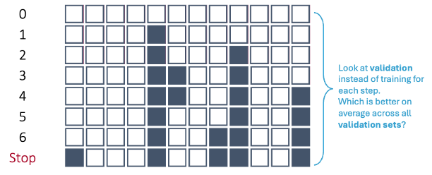{fig-align="center" width="8in"}In first step of the stepwise selection process, we create models such that each model has exactly one predictor variable and calculate a model metric for each model. However, we do this across **each cross-validation training set**. For 10-fold cross-validation, that would be 10 separate first steps that create models with only one variable. Next, we average the model metric across all cross-validation training sets to see which is the best variable. For example, the 5th variable is now the best **on average** across all of the cross-validation datasets based on our model metric, not just the training set overall.This same process is repeated across all of the steps until a final model is selected where adding any further variables does not improve the model based on the cross-validation model metrics. Remember, the difference between forward and stepwise selection is that we are also evaluating each variable added to the model at each step to see if deleting that variable improves the model metric.Let's see this in each software!::: {.panel-tabset .nav-pills}## PythonTo gain the needed functionality for cross-validation recursive feature addition or subtraction, we need to use the `mlxtend` package on top of `scikit-learn`. Specifically, we will use the `SequentialFeatureSelector` function from `mlxtend.feature_selection`. We will need to create our logistic regression object with the `LogisticRegression` function, not the `statsmodels.api` version with the `Logit` function. We need the `penalty = None` option to perform traditional logistic regression with no additional penalties (discussed in the Regularization section of the code deck). This object will be an input to our `SFS` function. We also need an additional step to improve the speed of the feature selection - scaling the data. This will help improve the speed of the maximum llikelihood optimization. To do this we will use the `StandardScaler` function from the `sklearn.processing` package. We will take the reduced data frame of the predictors, `X_reduced`, and input it into the `StandardScaler` object with the `fit_transform` function. This function unfortunately doesn't produce a data frame output so we have to turn this into a data frame with the `pandas``DataFrame` function with the `columns` option to define the same columns as we had with the reduced dataset.Now we can define our `SFS` function. In the `k_features` option we can put any integer value to set a certain number of features, the `"best"` option to pick the number of features that provides the best value of the model metric, or the `"parsimonious"` option to pick the number of features within one standard error of the true best model to try and make the model simpler. The `forward = True` option makes the function perform forward selection. The `floating = True` option means that once a variable is added it is evaluated at each step to be dropped out of the model - stepwise selection. The `scoring` option allows you to select your model metric. The options for a binary target variable are the accuracy, precision, recall, F1 score, area under the ROC curve (`roc_auc`), negative log loss, and negative Brier score. These will be covered in much further detail in the next section of the code deck on Model Assessment. The reason the last two are negative is that the function tries to maximize the optimization function. The `cv` option allows you to pick the number of cross-validation folds. Lastly, we just use the `fit` function with our predictor variables and target variable to fit the model. The variables are then printed below.```{python}#| warning: false#| error: false#| message: falsefrom mlxtend.feature_selection import SequentialFeatureSelector as SFSfrom sklearn.linear_model import LogisticRegressionfrom sklearn.preprocessing import StandardScalerscaler = StandardScaler()X_scaled = scaler.fit_transform(X_reduced)X_scaled_df = pd.DataFrame(X_scaled, columns = X_reduced.columns)logr = LogisticRegression(max_iter =1000, solver ='newton-cg', penalty =None) # Backward selection to find best subset of featuressfs = SFS(logr, k_features ="best", forward =True, floating =True, scoring ='roc_auc', cv =10)sfs = sfs.fit(X_scaled_df, y)# Get selected feature namesselected_features =list(sfs.k_feature_names_)print("Selected features:", selected_features)```Now we have variables determined by stepwise selection with cross-validation.## RTo gain the needed functionality for cross-validation recursive feature addition or subtraction, we need to use the `caret` package. Specifically, we will use the `train` function from `caret` package along with the `MASS` package. The `caret` function can not handle our target variable and predictor variables being in separate objects. Therefore, we first use `cbind` to combine the target variable as a column to the predictor variables dataframe. Now we can use the new dataframe to put into `caret` with the typical formula structure we have used previously. We also need to make our target variable a factor object using the `factor` function for the package to fit the correct model.The `method = "glmStepAIC"` option uses the `MASS` package and its stepwise selection capabilities. You can think of `caret` as more of a wrapper function that puts a cross-validation spin on other functions.The `glmStepAIC` function that does recursive feature elimination such as stepwise selection uses likelihood based metrics to selection variables. We will use two of the most common ones: AIC and BIC (can also be referred to as SBC).The AIC, or **Akaike Information Criterion**, was developed by statistician Hirotugu Akaike in the 1970’s and is defined by:$$AIC = n \log(\frac{SSE}{n}) + 2(p + 1)$$In this case, the $SSE$ is the sum of squared error from the model and $2(p+1)$ is the “penalty”, where $p$ is the number of variables in the model. A smaller AIC indicates a better model.BIC, also known as the **Bayesian Information Criterion** (also called SBC or **Schwarz Bayesian Information**) was first developed by Gideon E. Schwarz, also back in the 1970’s and is defined by:$$BIC = n \log(\frac{SSE}{n}) + (p+1)\log (n)$$In this case, “Likelihood” is the likelihood of the data and $(p+1)\log(n)$ is the “penalty”, where $p$ is the number of variables in the model and $n$ is the sample size. A smaller BIC indicates a better model. This is how variables are selected at each step in the stepwise selection.However, the `metric` option allows you to select your model metric across cross-validation training sets to pick the best one. The options for a binary target variable are controlled with the `summaryFuction` option in the `trainControl` function. The `trControl = trainControl(method = 'cv', number = 10))` option allows you to pick the number of cross-validation folds. That summary function allows different evaluation metrics. We can pick the F1 score, precision, recall, area under the ROC curve (`AUC`), and area under the precision-recall curve. Using other optoins in the `summaryFunction` provides even more possible metrics. We also have to specify the `fmaily = "binomial` option to build a logistic regression and the `direction = "both"` option to specify we want stepwise selection. The `results` object will display our final performance metric and the `summary` function will show a summary of the final model built.```{r}#| warning: false#| error: false#| message: falselibrary(caret)library(MASS)library(MLmetrics)set.seed(1234)df <-cbind(y, X_reduced)df$y <-factor(df$y, levels =c(0, 1), labels =c("no", "yes"))step_model <- caret::train(y ~ ., data = df,method ="glmStepAIC", family ="binomial",direction ="both",metric ="AUC",trControl =trainControl(method ="cv", number =10,classProbs =TRUE,summaryFunction = prSummary), trace =FALSE)step_model$resultssummary(step_model$finalModel)```Now we have variables determined by stepwise selection with cross-validation.:::## Backward SelectionLet's also revisit the backward selection approach with cross-validation.{fig-align="center" width="8in"}In first step of the backward selection process, we create models such that each model has exactly one predictor variable removed from it and calculate a model metric for each model. However, we do this across **each cross-validation training set**. For 10-fold cross-validation, that would be 10 separate first steps that create models removing only one variable. Next, we average the model metric across all training sets to see which is the worst variable. For example, the second variable is now the worst **on average** across all of the cross-validation datasets based on our model metric, not just the training set overall.This same process is repeated across all of the steps until a final model is selected where removing any further variables does not improve the model based on the cross-validation model metrics.Let's see this in each software!::: {.panel-tabset .nav-pills}## PythonTo gain the needed functionality for cross-validation recursive feature addition or subtraction, we need to use the `mlxtend` package on top of `scikit-learn`. Specifically, we will use the `SequentialFeatureSelector` function from `mlxtend.feature_selection`. We will need to create our logistic regression object with the `LogisticRegression` function, not the `statsmodels.api` version with the `Logit` function. We need the `penalty = None` option to perform traditional logistic regression with no additional penalties (discussed in the Regularization section of the code deck). This object will be an input to our `SFS` function. We also need an additional step to improve the speed of the feature selection - scaling the data. This will help improve the speed of the maximum llikelihood optimization. To do this we will use the `StandardScaler` function from the `sklearn.processing` package. We will take the reduced data frame of the predictors, `X_reduced`, and input it into the `StandardScaler` object with the `fit_transform` function. This function unfortunately doesn't produce a data frame output so we have to turn this into a data frame with the `pandas``DataFrame` function with the `columns` option to define the same columns as we had with the reduced dataset.Now we can define our `SFS` function. In the `k_features` option we can put any integer value to set a certain number of features, the `"best"` option to pick the number of features that provides the best value of the model metric, or the `"parsimonious"` option to pick the number of features within one standard error of the true best model to try and make the model simpler. The `forward = False` and `floating = False` options makes the function perform backward selection. The `scoring` option allows you to select your model metric. The options for a binary target variable are the accuracy, precision, recall, F1 score, area under the ROC curve (`roc_auc`), negative log loss, and negative Brier score. These will be covered in much further detail in the next section of the code deck on Model Assessment. The reason the last two are negative is that the function tries to maximize the optimization function. The `cv` option allows you to pick the number of cross-validation folds. Lastly, we just use the `fit` function with our predictor variables and target variable to fit the model. The variables are then printed below.```{python}#| warning: false#| error: false#| message: falsefrom mlxtend.feature_selection import SequentialFeatureSelector as SFSfrom sklearn.linear_model import LogisticRegressionfrom sklearn.preprocessing import StandardScalerscaler = StandardScaler()X_scaled = scaler.fit_transform(X_reduced)X_scaled_df = pd.DataFrame(X_scaled, columns = X_reduced.columns)logr = LogisticRegression(max_iter =1000, solver ='newton-cg', penalty =None) # Backward selection to find best subset of featuressfs = SFS(logr, k_features ="best", forward =False, floating =False, scoring ='roc_auc', cv =10)sfs = sfs.fit(X_scaled_df, y)# Get selected feature namesselected_features =list(sfs.k_feature_names_)print("Selected features:", selected_features)```Now we have variables determined by backward selection using cross-validation. Let's see this final model using its variables in the traditional `Logit` function from `statsmodels`.```{python}#| warning: false#| error: false#| message: falseimport statsmodels.api as smX_selected = X_reduced[selected_features]# Build Logistic Regressionmodel = sm.Logit(y, X_selected)result = model.fit()print(result.summary())```Most of the variables are similar to the ones we had from stepwise selection with some slight variations.## RTo gain the needed functionality for cross-validation recursive feature addition or subtraction, we need to use the `caret` package. Specifically, we will use the `train` function from `caret` package along with the `MASS` package. The `caret` function can not handle our target variable and predictor variables being in separate objects. Therefore, we first use `cbind` to combine the target variable as a column to the predictor variables dataframe. Now we can use the new dataframe to put into `caret` with the typical formula structure we have used previously. We also need to make our target variable a factor object using the `factor` function for the package to fit the correct model.The `method = "glmStepAIC"` option uses the `MASS` package and its backward selection capabilities. You can think of `caret` as more of a wrapper function that puts a cross-validation spin on other functions. The `glmStepAIC` function that does recursive feature elimination such as backward selection uses likelihood based metrics to selection variables just like we discussed with the stepwise selection above.However, the `metric` option allows you to select your model metric across cross-validation training sets to pick the best one. The options for a binary target variable are controlled with the `summaryFuction` option in the `trainControl` function. The `trControl = trainControl(method = 'cv', number = 10))` option allows you to pick the number of cross-validation folds. That summary function allows different evaluation metrics. We can pick the F1 score, precision, recall, area under the ROC curve (`AUC`), and area under the precision-recall curve. Using other optoins in the `summaryFunction` provides even more possible metrics. We also have to specify the `fmaily = "binomial` option to build a logistic regression and the `direction = "backward"` option to specify we want backward selection. The `results` object will display our final performance metric and the `summary` function will show a summary of the final model built.```{r}#| warning: false#| error: false#| message: falselibrary(caret)library(MASS)set.seed(1234)df <-cbind(y, X_reduced)df$y <-factor(df$y, levels =c(0, 1), labels =c("no", "yes"))back_model <- caret::train(y ~ ., data = df,method ="glmStepAIC", family ="binomial",direction ="backward",metric ="AUC",trControl =trainControl(method ="cv", number =10,classProbs =TRUE,summaryFunction = prSummary), trace =FALSE)back_model$resultssummary(back_model$finalModel)```Now we have variables determined by backward selection using cross-validation. Most of the variables are similar to the ones we had from stepwise selection with some slight variations.:::## Forward Selection with InteractionsHere we will work through forward selection. In forward selection, the initial model is empty (contains no variables, only the intercept). Each variable is then tried to see how much it improves a model based on a model metric. The most important variable (based on that metric) is then added to the model. Then the remaining variables are again tested and the next most impactful variable (based on the same model metric) is added to the model. This process repeats until either no more variables are available to add to the model based on the metric. This approach is the same as stepwise selection without the additional check at each step for possible removal.Forward selection is the least used technique because stepwise selection does the same as forward selection with the added benefit of dropping insignificant variables. The main use for forward selection is to test higher order terms and interactions in models. You can start with your model determined from either stepwise or backward selection and then try to add only interactions between variables from there.The code for this is not shown here, but it is a simple change to the code above to perform this approach.# Calibration CurvesAnother evaluation/diagnostic for logistic regression is the **calibration curve**. The calibration curve is a goodness-of-fit measure for logistic regression. Calibration measures how well predicted probabilities agree with actual frequency counts of outcomes (estimated linearly across the data set). These curves can help detect if predictions are consistently too high or low in your model.If the curve is above the diagonal line, this indicates the model is predicting **lower** probabilities than actually observed. The opposite is true if the curve is below the diagonal line.This is best used on larger samples since we are calculating the observed proportion of events in the data. In smaller samples this relationship is extrapolated out from the center and may not as accurately reflect the truth.Let's look at creating these in each software!::: {.panel-tabset .nav-pills}## PythonTo build a calibration curve in Python we can use the `calibration_curve` function inside of the `sklearn.calibration` package. The input to this function are the target variable, `bonus`, and our predicted probabilities from our data. To get these predicted values we can use the `predict` function on our model object called `result`. The inputs for this `predict` function are a dataset we want to score. We will calculate the predicted probabilities of our training dataset. The model we are using comes from the backward selection from above. The other options in the `calibration_curve` function in Python is how many bins you want to compute the goodness-of-fit (here we use 10) and the strategy for this calculation. We will use the `strategy = 'quantile'` option. This option breaks our data into 10 groups of equal sizes of observations instead of just splitting the probabilities into groups of 0-0.1, 0.1-0.2, etc.The `calibration_curve` function produces two outputs - the fraction of positives in each bin (the true probability) and the average predicted probability of each bin. These should be close to each other for the model to be well calibrated. The rest of the code is just used to plot this calibration curve.```{python}#| warning: false#| error: false#| message: falsefrom sklearn.calibration import calibration_curvetrain['pred_prob'] = result.predict(X_selected)# Compute calibration curveprob_true, prob_pred = calibration_curve(train['bonus'], train['pred_prob'], n_bins =10, strategy ='quantile')plt.figure(figsize = (6, 6))plt.plot(prob_pred, prob_true, marker ='o', label ='Calibration curve')plt.plot([0, 1], [0, 1], linestyle ='--', color ='gray', label ='Perfectly calibrated')plt.xlabel('Predicted probability')plt.ylabel('Observed frequency')plt.title('Calibration Curve')plt.legend()plt.grid(True)plt.tight_layout()plt.show()```Since the calibration curve line is consistently along the straight line, we do not notice any significant number of over or under predictions.## RR produces a calibration curve using the `givitiCalibrationBelt` function. The inputs to this function are `o =` and `e =`. These are the observed target and expected (predicted) target respectively. To get these predicted values we can use the `predict` function on our model object called `back_model`. We will calculate the predicted probabilities of our training dataset. The model we are using comes from the backward selection from above. We place our actual target variable in the `o =` option and the predictions from our logistic regression model in the `e =` option. Since the model is being compared to training data the `devel = internal` option is specified. The `maxDeg =` option sets the maximum degree being tested for the curve.```{r}#| warning: false#| error: false#| message: falselibrary(givitiR)cali.curve <-givitiCalibrationBelt(o = train$bonus,e =predict(back_model, type ="prob")[, "yes"],devel ="internal",maxDeg =5)plot(cali.curve, main ="Bonus Eligibility Model Calibration Curve",xlab ="Predicted Probability",ylab ="Observed Bonus Eligibility")```Since the diagonal line is contained in the confidence interval for our calibration curve, we do not notice any significant number of over or under predictions.:::# Diagnostic PlotsLinear regression models contain residuals with properties that are very useful for model diagnostics. However, what is a residual in a logistic regression model? Since we don’t have actual probabilities to compare our predicted probabilities against, residuals are not as clearly defined. Instead we have pseudo “residuals” in logistic regression that we can explore further. Two examples of this are **deviance residuals** and **Pearson residuals**.Deviance is a measure of how far a fitted model is from the fully saturated model. The fully saturated model is a model that predicts our data perfectly by essentially overfitting to it - a variable for each unique combination of inputs. This makes this model impractical for use, but good for comparison. The deviance is essentially our “error” from this “perfect” model. Logistic regression minimizes the sum of the squared deviances. Deviance residuals tell us how much each observation reduces the deviance.Pearson residuals on the other hand tell us how much each observation changes the Pearson Chi-squared test for the overall model.Other forms of measuring an observation’s influence on the logistic regression model are **DFBetas** and **Cook’s D**. Similar to their interpretation in linear regression, these two calculations tell us how each observation changes the estimation of each parameter individually (DFBeta) or how each observation changes the estimation of all the parameters holistically (Cook’s D).Let’s see how to get all of these from each software!::: {.panel-tabset .nav-pills}## PythonPython has some wonderful diagnostics plots to show us these residuals. Python also produces a list of these measures of influence as well as many more with the `get_influence` function. Below only the first 5 observations are shown using the `head` function, but this is calculated for each of the observations.```{python}#| warning: false#| error: false#| message: falseinfluence = result.get_influence()influence.summary_frame().head()```The output above has all of the needed information. We can get both Cook's D and DFBeta's from the above summary as well as many other metrics. The following code just takes the Cook's D values and DFBeta values and plots them. Only one of the DFBetas plots is actually shown.```{python}#| warning: false#| error: false#| message: false#| eval: falsedfbetas = influence.dfbetasn_obs, n_params = dfbetas.shapeparam_names = result.params.index# Rule-of-thumb thresholdthreshold =2/ np.sqrt(n_obs)for i inrange(n_params): plt.figure(figsize=(8, 4)) plt.stem(dfbetas[:, i]) plt.axhline(threshold, color='red', linestyle='--') plt.axhline(-threshold, color='red', linestyle='--') plt.title(f'DFBETAs for {param_names[i]}') plt.xlabel('Observation index') plt.ylabel('DFBETA') plt.grid(True) plt.show()``````{python}#| warning: false#| error: false#| message: false#| echo: falsedfbetas = influence.dfbetasn_obs, n_params = dfbetas.shapeparam_names = result.params.indexparam ="GrLivArea"# or whatever your variable name isindex =list(param_names).index(param)dfbeta_var = dfbetas[:, index]# Rule-of-thumb thresholdn =len(dfbeta_var)threshold =2/ np.sqrt(n)plt.figure(figsize=(10, 4))plt.stem(dfbeta_var)plt.axhline(y=threshold, color='red', linestyle='--', label='Threshold')plt.axhline(y=-threshold, color='red', linestyle='--')plt.title(f'DFBETAs for variable: {param}')plt.xlabel('Observation index')plt.ylabel('DFBETA')plt.legend()plt.grid(True)plt.show()``````{python}#| warning: false#| error: false#| message: falsecooks_d = influence.cooks_distance[0]n =len(cooks_d)threshold =4/ nplt.figure(figsize=(10, 4))plt.stem(cooks_d)plt.axhline(y=threshold, color='red', linestyle='--', label=f'Threshold (4/n = {threshold:.4f})')plt.title("Cook's Distance for Each Observation")plt.xlabel('Observation Index')plt.ylabel("Cook's Distance")plt.legend()plt.grid(True)plt.show()```## RR has some wonderful diagnostics plots to show us these residuals. R also produces a list of these measures of influence as well as many more with the `influence.measures` function. Below only the first 6 observations are shown using the `head` function, but this is calculated for each of the observations. The 4th plot in the `plot` function on the logistic regression model object is the Cook’s D plot as shown below. The `dfbetasPlots` function produces the DFBetas plots, but only one is shown here.```{r}#| warning: false#| error: false#| message: falsefinal_vars <-names(coef(step_model$finalModel))final_vars <-setdiff(final_vars, "(Intercept)")final_formula <-as.formula(paste("y_numeric ~", paste(final_vars, collapse =" + ")))y_numeric <-ifelse(y =="yes", 1, 0)df_numeric <-cbind(y_numeric, X_reduced)glm_model <-glm(final_formula, data = df_numeric, family = binomial)``````{r}#| warning: false#| error: false#| message: falselibrary(car)head(influence.measures(glm_model)$infmat)plot(glm_model, 4)``````{r}#| warning: false#| error: false#| message: falsedfbetasPlots(glm_model, terms ="GrLivArea", id.n =5,col =ifelse(glm_model$y ==1, "red", "blue"))```:::