Linear models and regression-based modeling has many different forms and variations to try and predict a target variable. Tree-based frameworks to modeling are a different approach. A decision tree is a supervised learning algorithm built by recursively splitting the data into successively purer subsets of data that resemble a decision-making process (decision tree).
Data is split based on groupings of predictor variable values. Although algorithms exist that can do multi-way splits, the focus here will be on binary splits - just splitting the data into two groups. These trees are useful for predicting either continuous or categorical target variables.
Let’s look at an example with a continuous target variable. We are going to predict a target variable y with one predictor variable X using a decision tree algorithm.
We must split the data into 2 pieces based on the values of X. Here are all of the possible splits:
Let’s split the data in the first split point on the left hand side - an X value of 1.5. That would mean we have two groups - A and B.
The predictions from group A would be the average of the values of our target variable y from group A, \(\hat{y} = 2\). The predictions of group B would be the average of y from group B, \(\hat{y} = 5.5\).
Splitting
The main question is how we choose the best split. Splitting is done based on some condition. The classification and regression tree (CART) approach to decision trees uses mean square error (MSE) to decide the best split for continuous target variables and measurements of purity like Gini or entropy for classification target variables. The chi-square automatic interaction detector (CHAID) approach to decision trees uses \(\chi^2\) tests and p-values to determine the best split.
Let’s continue the above example with the CART approach to decision trees. We will make the best split based on MSE. We want a split that will minimize the MSE for our predictions. Since we have the predictions for the first split above, let’s calculate the MSE for each group:
Now let’s move the split to the next possible location, 2.5:
Now our predictions for group A and B are \(3\) and \(6\) respectively. Let’s again calculate the MSE for each group and the overall MSE for the split at 2.5:
This split has a lower overall MSE than the first split. In fact, if we were to continue this process for every split we would see that this split is the best of all possible binary splits.
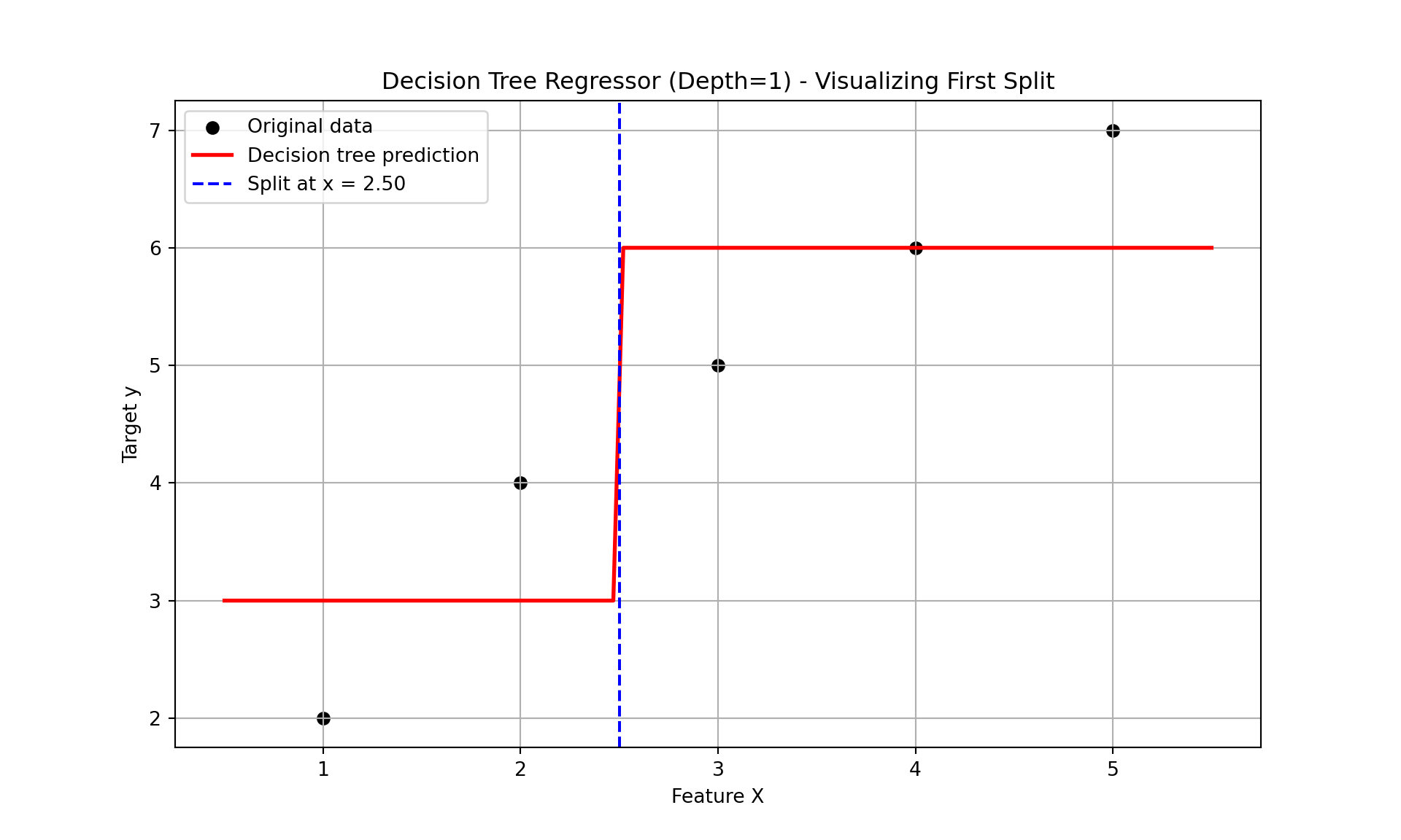
Now we have our best decision tree model if we were to limit ourselves to splitting our data only once. Since our predictions are just the average of each group, we have a step function for our model as we can see below:
DecisionTreeRegressor(max_depth=1)
In a Jupyter environment, please rerun this cell to show the HTML representation or trust the notebook. On GitHub, the HTML representation is unable to render, please try loading this page with nbviewer.org.
Parameters
criterion
'squared_error'
splitter
'best'
max_depth
1
min_samples_split
2
min_samples_leaf
1
min_weight_fraction_leaf
0.0
max_features
None
random_state
None
max_leaf_nodes
None
min_impurity_decrease
0.0
ccp_alpha
0.0
monotonic_cst
None
Split Threshold: 2.5
Left Node Prediction: [[3.]]
Right Node Prediction: [[6.]]
Let’s see how to build a simple CART decision tree in each software!
Building a CART decision tree in Python is rather simple. First, let’s create the same dataset that we have been working with above by creating two arrays with the numpyarray function. Next, we just need the DecisionTreeRegressor function from the sklearn.tree package. We will set the max_depth option to 1 so that we will only find one split. Lastly, we just put the data arrays into the fit function and we have our model.
Code
import numpy as npimport matplotlib.pyplot as pltfrom sklearn.tree import DecisionTreeRegressor# Simple regression datasetX_little = np.array([[1], [2], [3], [4], [5]])y_little = np.array([2, 4, 5, 6, 7])# Fit regression tree with max_depth = 1 (only one split)model = DecisionTreeRegressor(max_depth =1)model.fit(X_little, y_little)
DecisionTreeRegressor(max_depth=1)
In a Jupyter environment, please rerun this cell to show the HTML representation or trust the notebook. On GitHub, the HTML representation is unable to render, please try loading this page with nbviewer.org.
Parameters
criterion
'squared_error'
splitter
'best'
max_depth
1
min_samples_split
2
min_samples_leaf
1
min_weight_fraction_leaf
0.0
max_features
None
random_state
None
max_leaf_nodes
None
min_impurity_decrease
0.0
ccp_alpha
0.0
monotonic_cst
None
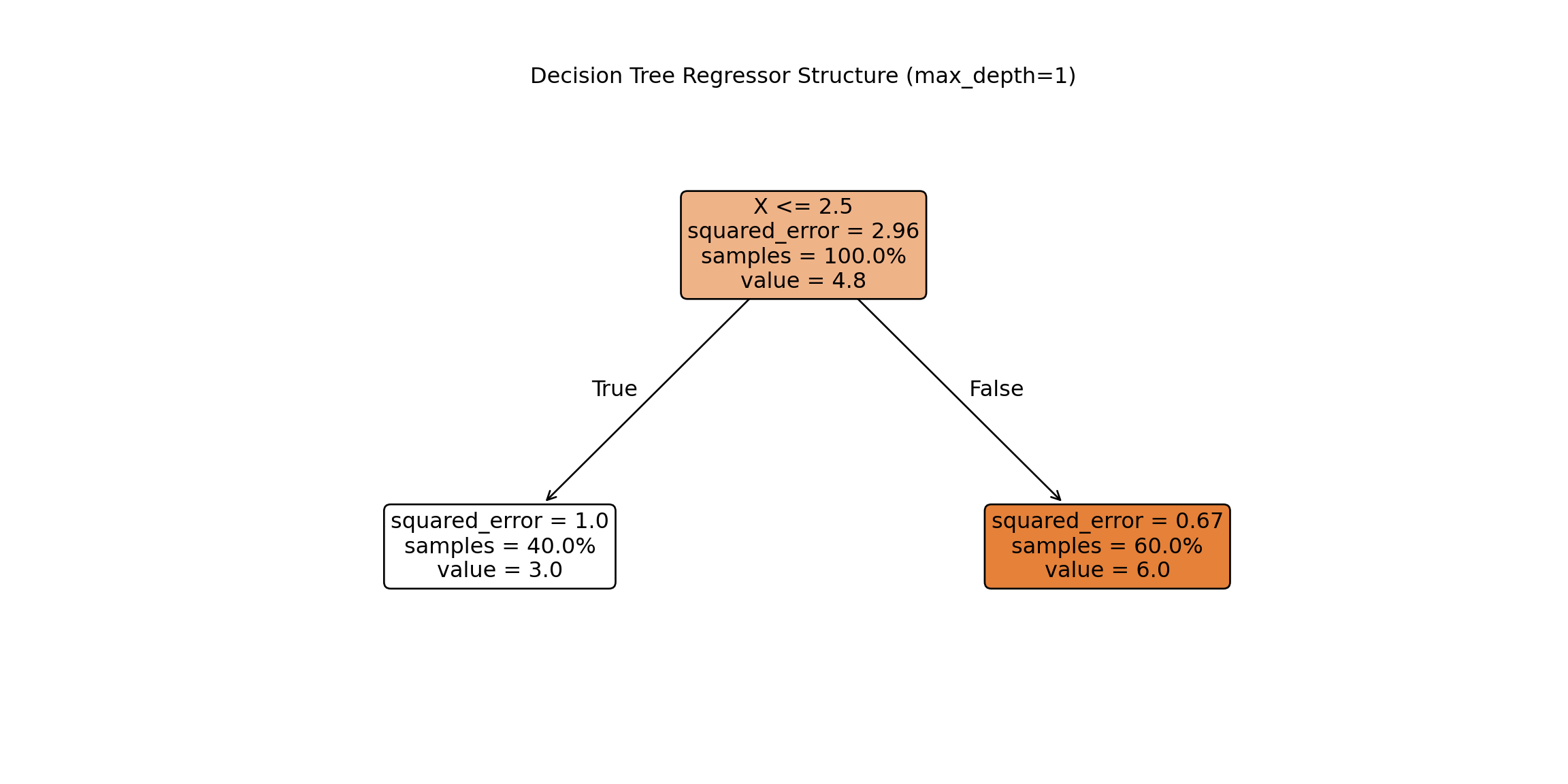
Unlike a linear regression, a decision tree’s output is much more visual in nature. To do view the decision tree we can use the plot_tree function from the sklearn.tree package. The input to the plot_tree function is the decision tree model object from above. Most of the options are aesthetic in nature. However, the feature_names option is useful to see the actual variable names and the proportion option is used to show the proportion of the data in each node instead of raw counts.
From the above figure of the decision tree we can see the same structure and calculations we did by hand. The split is listed right at the top with the X variable optimally split at 2.5. In each piece we see the squared error on each side of the split, the percentage of observations in that split, and the predicted value in that piece of the split as well. Notice how the squared error, percentage of observations, and predicted values are exactly as calculated above.
Building a CART decision tree in R is rather simple. First, let’s create the same dataset that we have been working with above by creating a data frame with the data.frame function and a vector with a c function. Next, we just need the rpart function from the rpart package. We will set the max_depth option to 1 so that we will only find one split. Lastly, we just put the data into the rpart function using the typical formula framework. The method = "anova" option specifies that we will use MSE as our split decider. The cp, minsplit, and minbucket options were set to their smallest values since our toy example only had 5 observations.
Code
library(rpart)X_little <-data.frame(x =c(1, 2, 3, 4, 5))y_little <-c(2, 4, 5, 6, 7)# Fit regression tree with maxdepth = 1 (only one split)model <-rpart(y_little ~ x, data = X_little, method ="anova", # "anova" is used for regressioncontrol =rpart.control(maxdepth =1, cp =0, minsplit =1, minbucket =1))# Print summary of the modelprint(model)
Unlike a linear regression, a decision tree’s output is much more visual in nature. To do view the decision tree we can use the rpart.plot function from the rpart.plot package. The input to the rpart.plot function is the decision tree model object from above. Most of the options are aesthetic in nature.
Code
library(rpart.plot)# Plot the decision treerpart.plot( model,type =2, extra =101, under =TRUE, faclen =0, fallen.leaves =TRUE,main ="Decision Tree Regressor Structure (max_depth = 1)",roundint =FALSE, digits =2, box.palette ="GnBu")
From the above figure of the decision tree we can see the same structure and calculations we did by hand. The split is listed right at the top with the X variable optimally split at 2.5. In each piece we see the percentage of observations in that split and the predicted value in that piece of the split as well. Notice how the percentage of observations and predicted values are exactly as calculated above.
The exact same process would occur if we wanted to go 2 levels deep into our decision tree. Each piece of the decision tree would have the same process to see if additional splits within each of group A or group B would help improve the model’s MSE. The predictions for a 2 level decision tree would be a more complicated step function as seen below:
In a Jupyter environment, please rerun this cell to show the HTML representation or trust the notebook. On GitHub, the HTML representation is unable to render, please try loading this page with nbviewer.org.
Adjusting the code to a 2 level decision tree in Python is just an adjustment to the max_depth option.
Code
import numpy as npimport matplotlib.pyplot as pltfrom sklearn.tree import DecisionTreeRegressor# Simple regression datasetX_little = np.array([[1], [2], [3], [4], [5]])y_little = np.array([2, 4, 5, 6, 7])# Fit regression tree with max_depth = 2 (only two splits)model = DecisionTreeRegressor(max_depth =2)model.fit(X, y)
DecisionTreeRegressor(max_depth=2)
In a Jupyter environment, please rerun this cell to show the HTML representation or trust the notebook. On GitHub, the HTML representation is unable to render, please try loading this page with nbviewer.org.
The top node of the decision tree is referred to commonly as the root node. The very bottom nodes are sometimes called leaves or terminal nodes. Nodes can also be referred to as parent and children nodes. Children nodes are a level below their corresponding parent node.
Adjusting the code to a 2 level decision tree in R is just an adjustment to the max_depth option.
Code
library(rpart)X_little <-data.frame(x =c(1, 2, 3, 4, 5))y_little <-c(2, 4, 5, 6, 7)# Fit regression tree with maxdepth = 1 (only one split)model <-rpart(y_little ~ x, data = X_little, method ="anova", # "anova" is used for regressioncontrol =rpart.control(maxdepth =2, cp =0, minsplit =1, minbucket =1))# Print summary of the modelprint(model)
library(rpart.plot)# Plot the decision treerpart.plot( model,type =2, extra =101, under =TRUE, faclen =0, fallen.leaves =TRUE,main ="Decision Tree Regressor Structure (max_depth = 1)",roundint =FALSE, digits =2, box.palette ="GnBu")
The top node of the decision tree is referred to commonly as the root node. The very bottom nodes are sometimes called leaves or terminal nodes. Nodes can also be referred to as parent and children nodes. Children nodes are a level below their corresponding parent node.
Attributes
One of the major reasons why decision trees are such a popular algorithm is that they are interpretable. With a series of binary decisions, you can easily follow why a prediction is the way that it is. You can also see if that specific split increases or decreases a prediction. These binary decisions are also very easy to implement into a system that scores customers.
The models of decision trees are also more complicated than one might realize from an initial look at them. Decision trees and the step functions they produce for predictions are not limited to linear associations. The prediction of each final split is just the average of all of the observations in that group. This means the pattern could easily be nonlinear and that wouldn’t impact the predictions from the decision tree. Each decision tree is also full of interactions between variables. Since each subsequent split after the first split is within each group, that implies that different groups after a split could be impacted differently by different variables. For example, A categorical X2 variable might be important to split values below 2.5 from the variable X, but not values above 2.5.
That previous point about variable splits impacting the decisions of variable splits after them implies that decision trees are greedy algorithms. Greedy algorithms makes the locally optimal choice at each step with the hope that these local decisions lead to a globally optimal solution. However, the decision tree only picks the next best option and doesn’t go back to reconsider the choice after looking at the next decision points. This means there is not a guarantee of an optimal solution.
Tuning / Optimizing Decision Trees
With multiple variables, every variable is evaluated at every split to find the “best” single split across all possible splits across all possible variables. This includes categorical variables that have been dummy coded and each dummy coded variable is evaluated separately.
With all of these variables and possible splits we have to worry about over-fitting our data. To prevent over-fitting of our data there are some common factors in a CART decision tree we can tune:
Max depth of tree - how many split levels overall in the tree
Minimum samples in split - how many observations must be in a node to even try to split
Minimum samples in leaf - how many observations left over in a leaf for a split to happen
When it comes to tuning machine learning models like decision trees there are many options for tuning. Cross-validation should be included in each of these approaches. Two of the most common tuning approaches are:
Grid search
Bayesian optimization
Grid search algorithms look at a fixed grid of values for each parameter you can tune - called hyperparameters. This means that every possible combination of values no matter is they are good or bad as it doesn’t learn from previous results. This is good for small samples with limited number of variables as it can be time consuming.
Bayesian optimization on the other hand is typically less computationally expensive as a grid search approach. The Bayesian optimization approach starts with random values for each hyperparameter you need to tune. It then fits a probabilistic model (a type of sequential model-based optimization) that “learns” the relationship between the parameters and performance. This process tries to estimate which hyperparameters are likely to produce good results and point it in the “correct” direction for values of hyperparameters. The next step in the optimization essentially “learns” from the previous combinations of hyperparameters. This approach is much more valuable for large samples with large numbers of variables.
We will continue to use our Ames housing dataset where we are predicting the sale price of a home. Even with tree-based algorithms, we still need to take the same steps to clean our data and do initial variable screening with business logic, low variability, missingness, and single variable comparison to the target. Machine learning models don’t protect you to a point where you can just throw in horrible data!
In Python we will build and tune decision trees with both a grid search and Bayesian optimization approach to compare.
Let’s start with the grid search approach. We will use the GridSearchCV and KFold functions from the sklearn.model_selection package. The first thing we do is define the range of values for the grid search across each of the hyperparameters we want to tune. We will tune the options max_depth, min_samples_split, and min_samples_leaf which correspond to the above hyperparameters commonly tuned in decision trees. The GridSearchCV function will basically rerun the DecisionTreeRegressor function with each unique combination of values defined in the grid of hyperparameters. The list and range functions help put in values for those options. The KFold function defines the cross-validation that we will use. We will use a 10-fold cross-validation. The DecisionTreeRegressor model object, the parameter grid object, and cross-validation object are all inputs in the GridSearchCV function. The last thing to define is the scoring option where we will specify that we want to optimize the MSE. Specifically in Python, we optimize the negative MSE because it is a maximization algorithm instead of a minimization one.
Once the grid search object is defined we just use the fit function along with our data to optimize the model. The best_params_ function gives us the optimal combination of hyperparameters.
In a Jupyter environment, please rerun this cell to show the HTML representation or trust the notebook. On GitHub, the HTML representation is unable to render, please try loading this page with nbviewer.org.
# Best estimator and scoreprint("Best Regressor Params:", grid_search_reg.best_params_)
Best Regressor Params: {'max_depth': 6, 'min_samples_leaf': 2, 'min_samples_split': 16}
The best parameters according to the grid search are a max depth of 6, minimum samples per split of 16, and minimum samples per leaf at 2.
Let’s now build with Bayesian optimization. This involves slightly more complicated coding. First we must define our objective function where we similarly define our grid that we want to define. We will use the same hyperparameter values. We will still use the same DecisionTreeRegressor function as our grid search as well as the same Kfold function. The main differences come with the create_study function. This sets up the parameters previously defined with the objective. The direction option is used to tell the Bayesian optimization whether to maximize or minimize the outcome. The sampler option is where we control the seeding to make the optimization replicable. Inside of the sampler option we put in the samplers.TPESampler function with the seed set. Lastly, we use the optimize function with the defined objective on the create_study object. The best_params function gives us the optimal parameters from the Bayesian optimization.
Code
import optunafrom sklearn.tree import DecisionTreeRegressorfrom sklearn.model_selection import cross_val_score, train_test_splitfrom sklearn.metrics import mean_squared_error# Define the Optuna objective functiondef objective(trial): max_depth = trial.suggest_int("max_depth", 2, 20) min_samples_split = trial.suggest_int("min_samples_split", 2, 20) min_samples_leaf = trial.suggest_int("min_samples_leaf", 1, 10) dt = DecisionTreeRegressor( max_depth=max_depth, min_samples_split=min_samples_split, min_samples_leaf=min_samples_leaf, random_state=1234 )# Use negative MSE (Optuna tries to maximize the return value) cv = KFold(n_splits =10, shuffle =True, random_state =1234) score = cross_val_score(dt, X_reduced, y, cv=cv, scoring="neg_mean_squared_error")return score.mean() # This is negative MSE# Run Optuna studysampler = optuna.samplers.TPESampler(seed=1234)study = optuna.create_study(direction="maximize", sampler=sampler) # Because we're maximizing negative MSEstudy.optimize(objective, n_trials=50)# Resultsprint("Best Parameters:", study.best_params)
Best Parameters: {'max_depth': 6, 'min_samples_split': 19, 'min_samples_leaf': 2}
The best parameters according to the grid search are a max depth of 6, minimum samples per split of 19, and minimum samples per leaf at 2. This was calculated in a fraction of the time of the grid search.
Let’s build our optimized decision tree on our training dataset using these last parameter values given to us by the Bayesian optimization.
In a Jupyter environment, please rerun this cell to show the HTML representation or trust the notebook. On GitHub, the HTML representation is unable to render, please try loading this page with nbviewer.org.
The tree plot above looks at the first two splits for our decision tree algorithm. The first split is on the overall quality of the home. The second split depends on the first split. If the overall quality of the home is high, then it looks at the square footage of the second floor. However, if the overall quality of the home is below 7.5 then it again splits on overall quality before looking at overall square footage.
In R we will build and tune decision trees with both a grid search and Bayesian optimization approach to compare.
Let’s start with the grid search approach. We will use the train and trainControl functions from the caret package. The first thing we do is define the range of values for the grid search across each of the hyperparameters we want to tune. In Python we have more control over the different tuning parameters we want in the decision tree as compared to R. With the rpart option inside of the train function we are only able to tune the cp option. The cp option controls the complexity parameter which corresponds to how much improvement we have to see in making a split. For example, a value of 0.01 would imply we need at least a 1% improvement for a split to occur. The train function will basically rerun the rpart function with each unique combination of values defined in the grid of hyperparameters. The expand.grid and seq functions help put in values for those options. The trainControl function defines the cross-validation that we will use. We will use a 10-fold cross-validation. The data, tuning grid, and cross-validation are all inputs to the train function. The last thing to define is the metric option where we will specify that we want to optimize the RMSE.
The bestTune element of the tuned model gives us the optimal combination of hyperparameters.
Code
library(caret)library(rpart)data <-data.frame(X_reduced, y = y)# Define the parameter gridgrid <-expand.grid(cp =seq(0.001, 0.05, by =0.001))# Define cross-validation folds (10-fold CV, shuffled)set.seed(1234)train_control <-trainControl(method ="cv", number =10)# Train the model using grid searchgrid_search_reg <-train( y ~ ., data = data,method ="rpart",trControl = train_control,tuneGrid = grid,metric ="RMSE")# Print best parametersprint(grid_search_reg$bestTune)
     cp
1 0.001
The best parameters according to the grid search are a complexity parameter of 0.001.
Let’s now build with Bayesian optimization. This involves slightly more complicated coding. First we must define our objective function where we similarly define our grid that we want to define. We will use the same hyperparameter values. We will still use the same rpart function as our grid search. The main differences come with the bayesOpt function. This sets up the parameters previously defined with the objective. The input to the bayesOpt function are all of the pieces we previously defined. The bounds option defines the specific values of the parameters we are tuning. The getBestPars function gives us the optimal parameters from the Bayesian optimization.
Code
library(rpart)library(ParBayesianOptimization)data <-data.frame(X_reduced, y = y)# Define scoring function for Bayesian optimizationscore_func <-function(maxdepth, minsplit, minbucket) {# Ensure parameters are integers maxdepth <-round(maxdepth) minsplit <-round(minsplit) minbucket <-round(minbucket)# Train rpart with internal cross-validation model <-rpart( y ~ ., data = data,method ="anova",control =rpart.control(maxdepth = maxdepth,minsplit = minsplit,minbucket = minbucket,cp =0, # disable pruning, we tune maxdepthxval =10# 10-fold CV ) ) best_cp_row <-which.min(model$cptable[,"xerror"]) cv_error <- model$cptable[best_cp_row, "xerror"]# ParBayesianOptimization maximizes Score, so return negative RMSElist(Score =-cv_error)}# Define bounds for hyperparametersbounds <-list(maxdepth =c(2L, 20L),minsplit =c(2L, 20L),minbucket =c(1L, 10L))set.seed(1234)opt_results <-bayesOpt(FUN = score_func,bounds = bounds,initPoints =5, iters.n =50, # number of Bayesian optimization iterationsacq ="ucb", # acquisition functionverbose =0)# Best parametersbest_params <-getBestPars(opt_results)print(best_params)
library(rpart.plot)# Plot the decision treerpart.plot( dt_ames,type =2, extra =101, under =TRUE, faclen =0, fallen.leaves =TRUE,main ="Decision Tree Regressor - Ames Housing Dataset",roundint =FALSE, digits =2, box.palette ="GnBu")
The tree plot above looks at our decision tree algorithm. The first split is on the overall quality of the home. The second split depends on the first split. If the overall quality of the home is high, then it looks at the square footage of the second floor. However, if the overall quality of the home is below 7.5 then it again splits on overall quality before looking at overall square footage.
Variable Importance
Most machine learning models are not interpretable in the classical sense - as one predictor variable increases, the target variable tends to ___. This is because the relationships are not linear. The relationships are more complicated than a linear relationship, so the interpretations are as well. Decision trees, however, are still interpretable based on the decision framework they are built with.
Although decision trees have an interpretable framework, we don’t have p-values like we do in statistical regression modeling to help us understand variable importance. Variable importance is a way of telling which variables “mean more” to the model than other variables.
In decision trees, the metric for variable importance is the MDI - mean decrease in impurity. Impurity has a different meaning depending on the type of target variable. In regression based trees with continuous target variables, the impurity metric is typically the variance of the residuals which is calculated by MSE. For classification based trees with a categorical target variable, the impurity metric is typically the Gini metric.
The MSE calculation has been used many times before in this code deck, however, the Gini impurity metric is new. Let’s look at its calculation:
\[
Gini = 1 - \sum_{i=1}^C p_i^2
\]
The calculation is quite simple. It calculates the proportion of each class in the target variable for the node and sums them together. This measure of impurity is a measure of disorder so we want lower values. Lower Gini impurity implies that the child nodes are “purer.”
Every time a feature is used to split a node, the software measures how much that split reduces the impurity. These reductions are accumulated across all trees for each feature (variable). These reductions are then normalized to sum to 1. The one problem with this approach is that it tends to overemphasize variables with many unique values because there are more places to split the variable.
Let’s calculate variable importance in each software!
Python automatically calculates the variable importance for decision trees as it build them. All we have to do is call the feature_importances_ function on our model object. We could just use the print function to then print out the importance numbers. We plot them using the seaborn package below after sorting the importance values with the sort_values function.
Code
import matplotlib.pyplot as pltimport seaborn as sns# Get feature importancesimportances = dt_ames.feature_importances_# Create a Series with feature names and their importance scores then sortfeature_importances = pd.Series(importances, index = X_reduced.columns)sorted_importances = feature_importances.sort_values(ascending =False)# Plotplt.figure(figsize=(8, len(sorted_importances) *0.3)) # dynamic heightsns.barplot(x=sorted_importances.values, y=sorted_importances.index)plt.title("Feature Importances from Decision Tree")plt.xlabel("Importance Score")plt.ylabel("Features")plt.tight_layout()plt.show()
As we can see from the plot above, The overall quality of the home is the dominant feature in terms of importance of predicting sales price. This is followed by total square footage of the living area, second floor square footage, and so on. Any variables that have an importance score of 0 were not used at all during the building of the decision tree.
R automatically calculates the variable importance for decision trees as it build them. All we have to do is call the variable.importance element on our model object. We could just use the print function to then print out the importance numbers. We plot them using the ggplot2 package below after sorting the importance values with the order function.
Models are nothing but potentially complicated formulas or rules. Once we determine the optimal model, we can score any new observations we want with the equation.
Scoring
It’s the process of applying a fitted model to input data to generate outputs like predicted values, probabilities, classifications, or scores.
Scoring data does not mean that we are re-running the model/algorithm on this new data. It just means that we are asking the model for predictions on this new data - plugging the new data into the equation and recording the output. This means that our data must be in the same format as the data put into the model. Therefore, if you created any new variables, made any variable transformations, or imputed missing values, the same process must be taken with the new data you are about to score.
For this problem we will score our test dataset that we have previously set aside as we were building our model. The test dataset is for comparing final models and reporting final model metrics. Make sure that you do NOT go back and rebuild your model after you score the test dataset. This would no longer make the test dataset an honest assessment of how good your model is actually doing. That also means that we should NOT just build hundreds of iterations of our same model to compare to the test dataset. That would essentially be doing the same thing as going back and rebuilding the model as you would be letting the test dataset decide on your final model.
Without going into all of the same detail as before, the following code transforms the test dataset we originally created in the same way that we did for the training dataset by dropping necessary variables, making missing value imputations, and getting our same data objects.
Code
predictors_test = test.drop(columns=['SalePrice'])ames_dummied = pd.get_dummies(ames, drop_first=True)test_ids = test.indextest_dummied = ames_dummied.loc[test_ids]predictors_test = test_dummied.astype(float)predictors_test = predictors_test.drop(['GarageType_Missing', 'GarageQual_Missing','GarageCond_Missing'], axis=1)# Impute Missing for Continuous Variablesnum_cols = predictors_test.select_dtypes(include='number').columnsfor col in num_cols:if predictors_test[col].isnull().any(): predictors_test[f'{col}_was_missing'] = predictors_test[col].isnull().astype(int)# Impute with median median = predictors_test[col].median() predictors_test[col] = predictors_test[col].fillna(median)X_test = predictors_testy_test = test['SalePrice']y_test_log = np.log(test['SalePrice'])# Subset the DataFrame to selected featuresX_test_selected = X_test[selected_features].copy()
Now that our data is ready for scoring we can use the predict function on our model object we created with our decision tree. The only input to the predict function is the dataset we prepared for scoring.
From the sklearn.metrics package we have a variety of model metric functions. We will use the mean_absolute_error (MAE) and mean_absolute_percentage_error (MAPE) metrics like the ones we described in the section on Model Building.
From the above output we can see that the linear regression model still beats thisd newly added decision tree.
Model
MAE
MAPE
Linear Regression
$18,160.24
11.36%
Ridge Regression
$19.572.19
12.25%
GAM
$18,154.31
11.40%
Decision Tree
$25,422.52
16.01%
To make sure that we are using the same test dataset between Python and R we will import our Python dataset here into R. There are a few variables that need to be renamed with the names function to work best in R.
Now that our data is ready for scoring we can use the predict function on our model object we created with our decision tree. The only input to the predict function is the dataset we prepared for scoring with the newdata option.
From the Metrics package we have a variety of model metric functions. We will use the mae (mean absolute error) and mape (mean absolute percentage error) metrics like the ones we described in the section on Model Building.
From the above output we can see that the linear regression model still beats this newly added decision tree.
Model
MAE
MAPE
Linear Regression
$18,160.24
11.36%
Ridge Regression
$22,040.76
13.37%
GAM
$19,479.79
12.23%
Decision Tree
$22,934.49
13.92%
Summary
In summary, decision tree models are interpretable, decision based framework models. Some of the advantages of using decision trees:
Computationally fast
Still interpretable due to decision framework output
Easy to implement
Variable importance provided
There are some disadvantages though:
Typically, not as predictive as more advanced models
Greedy algorithm means every decision is completely based on the previous decision
Bias towards features with more levels
Bagging
Before understanding the concept of bagging, we need to know what a bootstrap sample is. A Bootstrap sample is a random sample of your data with replacement that are the same size as your original data set. By random chance, some of the observations will not be sampled. These observations are called out-of-bag observations. Three example bootstrap samples of 10 observations labelled 1 through 10 are listed below:
Bootstrap Sample Examples
Mathematically, a bootstrap sample will contain approximately 63% of the observations in the data set. The sample size of the bootstrap sample is the same as the original data set, just some observations are repeated. Bootstrap samples are used in simulation to help develop confidence intervals of complicated forecasting techniques. Bootstrap samples are also used to ensemble models using different training data sets - called bagging.
Bootstrap aggregating (bagging) is where you take k bootstrap samples and create a model using each of the bootstrap samples as the training data set. This will build k different models. We will ensemble these k different models together.
Let’s work through an example to see the potential value. The following 10 observations have the values of X and Y shown in the following table:
We will build a decision stump (a decision tree with only one split). From building a decision stump, the best accuracy is obtained by making the split at either 3.5 or 7.5. Either of these splits would lead to an accuracy of predicting Y at 70%. For example, let’s use the split at 3.5. That would mean we think everything above 3.5 is a 0 and everything below 3.5 is a 1. We would get observations 1, 2, and 3 all correct. However, since everything above 3.5 is considered a 0, we would only get observations 4, 5, 6, and 7 correct on that piece - missing observations 8, 9, and 10.
To try and make this prediction better we will do the following:
Take 10 bootstrap samples
Build a decision stump for each
Aggregate these rules into a voting ensemble
Test the performance of the voting ensemble on the whole dataset
The following is the 10 bootstrap samples with their optimal splits. Remember, these bootstrap samples will not contain all of the observations in the original data set.
Some of these samples contain only one value of the target variable and so the predictions are the same for that bootstrap sample. However, we will use the optimal cut-offs from each of those samples to predict 1’s and 0’s for the original data set as shown in the table below:
Summary of Bootstrap Sample Predictions on Training Data
The table above has one row for each of the predictions from the 10 bootstrap samples. We can average these predictions of 1’s and 0’s together for each observation to get the average row near the bottom.
Let’s take a cut-off of 0.25 from our average values from the 1 and 0 predictions from each bootstrap sample. That would mean anything above 0.25 in the average row would be predicted as a 1 while everything below would be predicted as a 0. Based on those predictions (the Pred. row above) we get a perfect prediction compared to the true values of Y from our original data set.
In summary, bagging improves generalization error on models with high variance (simple tree-based models for example). If base classifier is stable (not suffering from high variance), then bagging can actually make predictions worse! Bagging does not focus on particular observations in the training data set (unlike boosting which is covered below).
Random Forests
Random forests are ensembles of decision trees (similar to the bagging example from above). Ensembles of decision trees work best when they find different patterns in the data. However, bagging tends to create trees that pick up the same pattern.
Random forests get around this correlation between trees by not only using bootstrapped samples, but also uses subsets of variables for each split and unpruned decision trees. For these unpruned trees, with a classification target it goes all the way until each unique observation is left in its own leaf. With regression trees the unpruned trees will continue until 5 observations are left per leaf. The results from all of these trees are ensembled together into one voting system. There are many choices of parameters to tune:
Let’s build a random forest with our Ames housing data set. We will use the RandomForestRegressor function from the sklearn.ensemble package. Similar to other Python functions we have used, we need the training predictor variables in one object and the target variable in another. The option to define how many decision trees are in the ensemble is n_estimators.
In a Jupyter environment, please rerun this cell to show the HTML representation or trust the notebook. On GitHub, the HTML representation is unable to render, please try loading this page with nbviewer.org.
Parameters
n_estimators
100
criterion
'squared_error'
max_depth
None
min_samples_split
2
min_samples_leaf
1
min_weight_fraction_leaf
0.0
max_features
1.0
max_leaf_nodes
None
min_impurity_decrease
0.0
bootstrap
True
oob_score
True
n_jobs
None
random_state
1234
verbose
0
warm_start
False
ccp_alpha
0.0
max_samples
None
monotonic_cst
None
The random_state option helps set the seed for the function to make the results repeatable. The oob_score = True option calculates the out-of-bag score for the model chosen for comparisons to other models of different sizes. For continuous targets it provides the \(R^2\) metric. For categorical targets this option provides the AUC. Let’s view that out-of-bag score with call of the oos_score_ element from the model object.
Code
rf_ames.oob_score_
0.8472859308068421
Let’s build a random forest with our Ames housing data set. We will use the randomForest function from the randomForest package. Similar to other R functions we have used, we need the training predictor variables in one object and the target variable in another. The option to define how many decision trees are in the ensemble is ntree.
Code
library(randomForest)set.seed(1234)# Fit random forestrf_ames <-randomForest(x = X_reduced,y = y,ntree =500, importance =TRUE, keep.inbag =TRUE)# Check OOB R^2print(rf_ames)
Call:
 randomForest(x = X_reduced, y = y, ntree = 500, importance = TRUE,      keep.inbag = TRUE)
               Type of random forest: regression
                     Number of trees: 500
No. of variables tried at each split: 15

          Mean of squared residuals: 966812021
                    % Var explained: 85.59
The set.seed option helps set the seed for the function to make the results repeatable. The importance = True option calculates the variable importance for the variables in the random forest. With the print function we can see the \(R^2\) of the model as the percentage of the variance explained.
Tuning / Optimizing Random Forests
There are a few things we can tune with a random forest. One is the number of trees used to build the model. Another thing to tune is the number of variables considered for each split - called mtry. By default, \(mtry = \sqrt{p}\), with \(p\) being the number of total variables. We can use cross-validation to tune these values. Just like with decision trees, we can use either a grid search approach or Bayesian optimization.
In Python we will build and tune random forests with both a grid search and Bayesian optimization approach to compare.
Let’s start with the grid search approach. In Python we can use the GridSearchCV function from the sklearn.model_selection package. In this function we need to define a grid to search across for the parameters to tune. Here are three common parameters to tune in the RandomForestRegressor function - max_depth which controls the depth of the trees, max_features which is mtry, and n_estimators which is the number of trees. The GridSearchCV function will basically rerun the RandomForestRegressor function with each unique combination of values defined in the grid of hyperparameters. The list and range functions help put in values for those options. The KFold function defines the cross-validation that we will use. We will use a 10-fold cross-validation. The RandomForestRegressor model object, the parameter grid object, and cross-validation object are all inputs in the GridSearchCV function. The last thing to define is the scoring option where we will specify that we want to optimize the MSE. Specifically in Python, we optimize the negative MSE because it is a maximization algorithm instead of a minimization one.
Once the grid search object is defined we just use the fit function along with our data to optimize the model. The best_params_ function gives us the optimal combination of hyperparameters.
In a Jupyter environment, please rerun this cell to show the HTML representation or trust the notebook. On GitHub, the HTML representation is unable to render, please try loading this page with nbviewer.org.
The best parameters according to the grid search are a max depth of 20, maximum number of features at 5, and 200 trees.
Let’s now build with Bayesian optimization. This involves slightly more complicated coding. First we must define our objective function where we similarly define our grid that we want to define. We will use the same hyperparameter values. We will still use the same RandomForestRegressor function as our grid search as well as the same Kfold function. The main differences come with the create_study function. This sets up the parameters previously defined with the objective. The direction option is used to tell the Bayesian optimization whether to maximize or minimize the outcome. The sampler option is where we control the seeding to make the optimization replicable. Inside of the sampler option we put in the samplers.TPESampler function with the seed set. Lastly, we use the optimize function with the defined objective on the create_study object. The best_params function gives us the optimal parameters from the Bayesian optimization.
Code
import optunafrom sklearn.model_selection import cross_val_scoreimport numpy as np# Step 1: Define the objective using a lambda so you keep your code flatdef objective(trial):# Define search space (equivalent to your param_grid) max_depth = trial.suggest_categorical('max_depth', [None, 10, 20, 30]) max_features = trial.suggest_int('max_features', 3, 7) n_estimators = trial.suggest_int('n_estimators', 100, 800, step=100)# Create the model with suggested parameters rf = RandomForestRegressor( max_depth = max_depth, max_features = max_features, n_estimators = n_estimators, random_state =1234 )# 10-fold CV like your original cv = KFold(n_splits =10, shuffle =True, random_state =1234) scores = cross_val_score(rf, X_reduced, y, cv = cv, scoring ='neg_mean_squared_error') # or 'r2'return np.mean(scores)# Step 2: Run the optimizationsampler = optuna.samplers.TPESampler(seed=1234)study = optuna.create_study(direction="maximize", sampler=sampler) # 'minimize' for error metricsstudy.optimize(objective, n_trials =50, show_progress_bar =True)
  0%|          | 0/50 [00:00<?, ?it/s]

[I 2025-11-15 22:22:36,982] Trial 0 finished with value: -943361450.4566427 and parameters: {'max_depth': 30, 'max_features': 6, 'n_estimators': 300}. Best is trial 0 with value: -943361450.4566427.

  0%|          | 0/50 [00:02<?, ?it/s]
Best trial: 0. Best value: -9.43361e+08:   0%|          | 0/50 [00:02<?, ?it/s]
Best trial: 0. Best value: -9.43361e+08:   2%|2         | 1/50 [00:02<02:11,  2.67s/it]

[I 2025-11-15 22:22:40,602] Trial 1 finished with value: -969205498.6342974 and parameters: {'max_depth': 20, 'max_features': 4, 'n_estimators': 500}. Best is trial 0 with value: -943361450.4566427.

Best trial: 0. Best value: -9.43361e+08:   2%|2         | 1/50 [00:06<02:11,  2.67s/it]
Best trial: 0. Best value: -9.43361e+08:   2%|2         | 1/50 [00:06<02:11,  2.67s/it]
Best trial: 0. Best value: -9.43361e+08:   4%|4         | 2/50 [00:06<02:35,  3.23s/it]

[I 2025-11-15 22:22:41,260] Trial 2 finished with value: -965598278.948608 and parameters: {'max_depth': 10, 'max_features': 5, 'n_estimators': 100}. Best is trial 0 with value: -943361450.4566427.

Best trial: 0. Best value: -9.43361e+08:   4%|4         | 2/50 [00:06<02:35,  3.23s/it]
Best trial: 0. Best value: -9.43361e+08:   4%|4         | 2/50 [00:06<02:35,  3.23s/it]
Best trial: 0. Best value: -9.43361e+08:   6%|6         | 3/50 [00:06<01:36,  2.06s/it]

[I 2025-11-15 22:22:42,824] Trial 3 finished with value: -1046005539.3524336 and parameters: {'max_depth': 10, 'max_features': 3, 'n_estimators': 300}. Best is trial 0 with value: -943361450.4566427.

Best trial: 0. Best value: -9.43361e+08:   6%|6         | 3/50 [00:08<01:36,  2.06s/it]
Best trial: 0. Best value: -9.43361e+08:   6%|6         | 3/50 [00:08<01:36,  2.06s/it]
Best trial: 0. Best value: -9.43361e+08:   8%|8         | 4/50 [00:08<01:25,  1.86s/it]

[I 2025-11-15 22:22:46,462] Trial 4 finished with value: -969122309.9938381 and parameters: {'max_depth': None, 'max_features': 4, 'n_estimators': 500}. Best is trial 0 with value: -943361450.4566427.

Best trial: 0. Best value: -9.43361e+08:   8%|8         | 4/50 [00:12<01:25,  1.86s/it]
Best trial: 0. Best value: -9.43361e+08:   8%|8         | 4/50 [00:12<01:25,  1.86s/it]
Best trial: 0. Best value: -9.43361e+08:  10%|#         | 5/50 [00:12<01:52,  2.50s/it]

[I 2025-11-15 22:22:51,735] Trial 5 finished with value: -946585642.9331744 and parameters: {'max_depth': None, 'max_features': 6, 'n_estimators': 600}. Best is trial 0 with value: -943361450.4566427.

Best trial: 0. Best value: -9.43361e+08:  10%|#         | 5/50 [00:17<01:52,  2.50s/it]
Best trial: 0. Best value: -9.43361e+08:  10%|#         | 5/50 [00:17<01:52,  2.50s/it]
Best trial: 0. Best value: -9.43361e+08:  12%|#2        | 6/50 [00:17<02:31,  3.44s/it]

[I 2025-11-15 22:22:52,776] Trial 6 finished with value: -1067759407.6078066 and parameters: {'max_depth': 10, 'max_features': 3, 'n_estimators': 200}. Best is trial 0 with value: -943361450.4566427.

Best trial: 0. Best value: -9.43361e+08:  12%|#2        | 6/50 [00:18<02:31,  3.44s/it]
Best trial: 0. Best value: -9.43361e+08:  12%|#2        | 6/50 [00:18<02:31,  3.44s/it]
Best trial: 0. Best value: -9.43361e+08:  14%|#4        | 7/50 [00:18<01:54,  2.66s/it]

[I 2025-11-15 22:22:55,363] Trial 7 finished with value: -1031545872.3392258 and parameters: {'max_depth': 10, 'max_features': 3, 'n_estimators': 500}. Best is trial 0 with value: -943361450.4566427.

Best trial: 0. Best value: -9.43361e+08:  14%|#4        | 7/50 [00:21<01:54,  2.66s/it]
Best trial: 0. Best value: -9.43361e+08:  14%|#4        | 7/50 [00:21<01:54,  2.66s/it]
Best trial: 0. Best value: -9.43361e+08:  16%|#6        | 8/50 [00:21<01:50,  2.64s/it]

[I 2025-11-15 22:22:56,171] Trial 8 finished with value: -947206379.641509 and parameters: {'max_depth': 30, 'max_features': 5, 'n_estimators': 100}. Best is trial 0 with value: -943361450.4566427.

Best trial: 0. Best value: -9.43361e+08:  16%|#6        | 8/50 [00:21<01:50,  2.64s/it]
Best trial: 0. Best value: -9.43361e+08:  16%|#6        | 8/50 [00:21<01:50,  2.64s/it]
Best trial: 0. Best value: -9.43361e+08:  18%|#8        | 9/50 [00:21<01:24,  2.06s/it]

[I 2025-11-15 22:23:02,840] Trial 9 finished with value: -947089933.7945614 and parameters: {'max_depth': 30, 'max_features': 7, 'n_estimators': 700}. Best is trial 0 with value: -943361450.4566427.

Best trial: 0. Best value: -9.43361e+08:  18%|#8        | 9/50 [00:28<01:24,  2.06s/it]
Best trial: 0. Best value: -9.43361e+08:  18%|#8        | 9/50 [00:28<01:24,  2.06s/it]
Best trial: 0. Best value: -9.43361e+08:  20%|##        | 10/50 [00:28<02:19,  3.49s/it]

[I 2025-11-15 22:23:05,691] Trial 10 finished with value: -952070764.9205726 and parameters: {'max_depth': 30, 'max_features': 7, 'n_estimators': 300}. Best is trial 0 with value: -943361450.4566427.

Best trial: 0. Best value: -9.43361e+08:  20%|##        | 10/50 [00:31<02:19,  3.49s/it]
Best trial: 0. Best value: -9.43361e+08:  20%|##        | 10/50 [00:31<02:19,  3.49s/it]
Best trial: 0. Best value: -9.43361e+08:  22%|##2       | 11/50 [00:31<02:08,  3.29s/it]

[I 2025-11-15 22:23:12,686] Trial 11 finished with value: -948786874.3366207 and parameters: {'max_depth': None, 'max_features': 6, 'n_estimators': 800}. Best is trial 0 with value: -943361450.4566427.

Best trial: 0. Best value: -9.43361e+08:  22%|##2       | 11/50 [00:38<02:08,  3.29s/it]
Best trial: 0. Best value: -9.43361e+08:  22%|##2       | 11/50 [00:38<02:08,  3.29s/it]
Best trial: 0. Best value: -9.43361e+08:  24%|##4       | 12/50 [00:38<02:47,  4.42s/it]

[I 2025-11-15 22:23:18,821] Trial 12 finished with value: -945913139.2376055 and parameters: {'max_depth': None, 'max_features': 6, 'n_estimators': 700}. Best is trial 0 with value: -943361450.4566427.

Best trial: 0. Best value: -9.43361e+08:  24%|##4       | 12/50 [00:44<02:47,  4.42s/it]
Best trial: 0. Best value: -9.43361e+08:  24%|##4       | 12/50 [00:44<02:47,  4.42s/it]
Best trial: 0. Best value: -9.43361e+08:  26%|##6       | 13/50 [00:44<03:02,  4.94s/it]

[I 2025-11-15 22:23:21,452] Trial 13 finished with value: -951154332.5193479 and parameters: {'max_depth': 20, 'max_features': 6, 'n_estimators': 300}. Best is trial 0 with value: -943361450.4566427.

Best trial: 0. Best value: -9.43361e+08:  26%|##6       | 13/50 [00:47<03:02,  4.94s/it]
Best trial: 0. Best value: -9.43361e+08:  26%|##6       | 13/50 [00:47<03:02,  4.94s/it]
Best trial: 0. Best value: -9.43361e+08:  28%|##8       | 14/50 [00:47<02:32,  4.24s/it]

[I 2025-11-15 22:23:28,460] Trial 14 finished with value: -948786874.3366207 and parameters: {'max_depth': None, 'max_features': 6, 'n_estimators': 800}. Best is trial 0 with value: -943361450.4566427.

Best trial: 0. Best value: -9.43361e+08:  28%|##8       | 14/50 [00:54<02:32,  4.24s/it]
Best trial: 0. Best value: -9.43361e+08:  28%|##8       | 14/50 [00:54<02:32,  4.24s/it]
Best trial: 0. Best value: -9.43361e+08:  30%|###       | 15/50 [00:54<02:57,  5.08s/it]

[I 2025-11-15 22:23:32,254] Trial 15 finished with value: -954726172.7552096 and parameters: {'max_depth': 30, 'max_features': 7, 'n_estimators': 400}. Best is trial 0 with value: -943361450.4566427.

Best trial: 0. Best value: -9.43361e+08:  30%|###       | 15/50 [00:57<02:57,  5.08s/it]
Best trial: 0. Best value: -9.43361e+08:  30%|###       | 15/50 [00:57<02:57,  5.08s/it]
Best trial: 0. Best value: -9.43361e+08:  32%|###2      | 16/50 [00:57<02:39,  4.69s/it]

[I 2025-11-15 22:23:37,077] Trial 16 finished with value: -957247928.1522877 and parameters: {'max_depth': None, 'max_features': 5, 'n_estimators': 600}. Best is trial 0 with value: -943361450.4566427.

Best trial: 0. Best value: -9.43361e+08:  32%|###2      | 16/50 [01:02<02:39,  4.69s/it]
Best trial: 0. Best value: -9.43361e+08:  32%|###2      | 16/50 [01:02<02:39,  4.69s/it]
Best trial: 0. Best value: -9.43361e+08:  34%|###4      | 17/50 [01:02<02:36,  4.73s/it]

[I 2025-11-15 22:23:43,205] Trial 17 finished with value: -945751162.0767119 and parameters: {'max_depth': 30, 'max_features': 6, 'n_estimators': 700}. Best is trial 0 with value: -943361450.4566427.

Best trial: 0. Best value: -9.43361e+08:  34%|###4      | 17/50 [01:08<02:36,  4.73s/it]
Best trial: 0. Best value: -9.43361e+08:  34%|###4      | 17/50 [01:08<02:36,  4.73s/it]
Best trial: 0. Best value: -9.43361e+08:  36%|###6      | 18/50 [01:08<02:44,  5.15s/it]

[I 2025-11-15 22:23:46,400] Trial 18 finished with value: -951557493.8687449 and parameters: {'max_depth': 30, 'max_features': 5, 'n_estimators': 400}. Best is trial 0 with value: -943361450.4566427.

Best trial: 0. Best value: -9.43361e+08:  36%|###6      | 18/50 [01:12<02:44,  5.15s/it]
Best trial: 0. Best value: -9.43361e+08:  36%|###6      | 18/50 [01:12<02:44,  5.15s/it]
Best trial: 0. Best value: -9.43361e+08:  38%|###8      | 19/50 [01:12<02:21,  4.56s/it]

[I 2025-11-15 22:23:48,318] Trial 19 finished with value: -957200046.0993801 and parameters: {'max_depth': 30, 'max_features': 7, 'n_estimators': 200}. Best is trial 0 with value: -943361450.4566427.

Best trial: 0. Best value: -9.43361e+08:  38%|###8      | 19/50 [01:14<02:21,  4.56s/it]
Best trial: 0. Best value: -9.43361e+08:  38%|###8      | 19/50 [01:14<02:21,  4.56s/it]
Best trial: 0. Best value: -9.43361e+08:  40%|####      | 20/50 [01:14<01:53,  3.77s/it]

[I 2025-11-15 22:23:52,679] Trial 20 finished with value: -966762463.3929113 and parameters: {'max_depth': 30, 'max_features': 4, 'n_estimators': 600}. Best is trial 0 with value: -943361450.4566427.

Best trial: 0. Best value: -9.43361e+08:  40%|####      | 20/50 [01:18<01:53,  3.77s/it]
Best trial: 0. Best value: -9.43361e+08:  40%|####      | 20/50 [01:18<01:53,  3.77s/it]
Best trial: 0. Best value: -9.43361e+08:  42%|####2     | 21/50 [01:18<01:54,  3.95s/it]

[I 2025-11-15 22:23:58,780] Trial 21 finished with value: -945751162.0767119 and parameters: {'max_depth': 30, 'max_features': 6, 'n_estimators': 700}. Best is trial 0 with value: -943361450.4566427.

Best trial: 0. Best value: -9.43361e+08:  42%|####2     | 21/50 [01:24<01:54,  3.95s/it]
Best trial: 0. Best value: -9.43361e+08:  42%|####2     | 21/50 [01:24<01:54,  3.95s/it]
Best trial: 0. Best value: -9.43361e+08:  44%|####4     | 22/50 [01:24<02:08,  4.59s/it]

[I 2025-11-15 22:24:04,923] Trial 22 finished with value: -945751162.0767119 and parameters: {'max_depth': 30, 'max_features': 6, 'n_estimators': 700}. Best is trial 0 with value: -943361450.4566427.

Best trial: 0. Best value: -9.43361e+08:  44%|####4     | 22/50 [01:30<02:08,  4.59s/it]
Best trial: 0. Best value: -9.43361e+08:  44%|####4     | 22/50 [01:30<02:08,  4.59s/it]
Best trial: 0. Best value: -9.43361e+08:  46%|####6     | 23/50 [01:30<02:16,  5.06s/it]

[I 2025-11-15 22:24:11,920] Trial 23 finished with value: -948593960.442934 and parameters: {'max_depth': 30, 'max_features': 6, 'n_estimators': 800}. Best is trial 0 with value: -943361450.4566427.

Best trial: 0. Best value: -9.43361e+08:  46%|####6     | 23/50 [01:37<02:16,  5.06s/it]
Best trial: 0. Best value: -9.43361e+08:  46%|####6     | 23/50 [01:37<02:16,  5.06s/it]
Best trial: 0. Best value: -9.43361e+08:  48%|####8     | 24/50 [01:37<02:26,  5.64s/it]

[I 2025-11-15 22:24:17,517] Trial 24 finished with value: -959292529.9675707 and parameters: {'max_depth': 30, 'max_features': 5, 'n_estimators': 700}. Best is trial 0 with value: -943361450.4566427.

Best trial: 0. Best value: -9.43361e+08:  48%|####8     | 24/50 [01:43<02:26,  5.64s/it]
Best trial: 0. Best value: -9.43361e+08:  48%|####8     | 24/50 [01:43<02:26,  5.64s/it]
Best trial: 0. Best value: -9.43361e+08:  50%|#####     | 25/50 [01:43<02:20,  5.63s/it]

[I 2025-11-15 22:24:23,229] Trial 25 finished with value: -950749246.7488773 and parameters: {'max_depth': 20, 'max_features': 7, 'n_estimators': 600}. Best is trial 0 with value: -943361450.4566427.

Best trial: 0. Best value: -9.43361e+08:  50%|#####     | 25/50 [01:48<02:20,  5.63s/it]
Best trial: 0. Best value: -9.43361e+08:  50%|#####     | 25/50 [01:48<02:20,  5.63s/it]
Best trial: 0. Best value: -9.43361e+08:  52%|#####2    | 26/50 [01:48<02:15,  5.65s/it]

[I 2025-11-15 22:24:26,746] Trial 26 finished with value: -940706820.8971512 and parameters: {'max_depth': 30, 'max_features': 6, 'n_estimators': 400}. Best is trial 26 with value: -940706820.8971512.

Best trial: 0. Best value: -9.43361e+08:  52%|#####2    | 26/50 [01:52<02:15,  5.65s/it]
Best trial: 26. Best value: -9.40707e+08:  52%|#####2    | 26/50 [01:52<02:15,  5.65s/it]
Best trial: 26. Best value: -9.40707e+08:  54%|#####4    | 27/50 [01:52<01:55,  5.01s/it]

[I 2025-11-15 22:24:29,958] Trial 27 finished with value: -951557493.8687449 and parameters: {'max_depth': 30, 'max_features': 5, 'n_estimators': 400}. Best is trial 26 with value: -940706820.8971512.

Best trial: 26. Best value: -9.40707e+08:  54%|#####4    | 27/50 [01:55<01:55,  5.01s/it]
Best trial: 26. Best value: -9.40707e+08:  54%|#####4    | 27/50 [01:55<01:55,  5.01s/it]
Best trial: 26. Best value: -9.40707e+08:  56%|#####6    | 28/50 [01:55<01:38,  4.47s/it]

[I 2025-11-15 22:24:31,718] Trial 28 finished with value: -950630085.5534309 and parameters: {'max_depth': 30, 'max_features': 6, 'n_estimators': 200}. Best is trial 26 with value: -940706820.8971512.

Best trial: 26. Best value: -9.40707e+08:  56%|#####6    | 28/50 [01:57<01:38,  4.47s/it]
Best trial: 26. Best value: -9.40707e+08:  56%|#####6    | 28/50 [01:57<01:38,  4.47s/it]
Best trial: 26. Best value: -9.40707e+08:  58%|#####8    | 29/50 [01:57<01:16,  3.66s/it]

[I 2025-11-15 22:24:36,462] Trial 29 finished with value: -950219295.9703524 and parameters: {'max_depth': 20, 'max_features': 7, 'n_estimators': 500}. Best is trial 26 with value: -940706820.8971512.

Best trial: 26. Best value: -9.40707e+08:  58%|#####8    | 29/50 [02:02<01:16,  3.66s/it]
Best trial: 26. Best value: -9.40707e+08:  58%|#####8    | 29/50 [02:02<01:16,  3.66s/it]
Best trial: 26. Best value: -9.40707e+08:  60%|######    | 30/50 [02:02<01:19,  3.98s/it]

[I 2025-11-15 22:24:39,693] Trial 30 finished with value: -951557493.8687449 and parameters: {'max_depth': 30, 'max_features': 5, 'n_estimators': 400}. Best is trial 26 with value: -940706820.8971512.

Best trial: 26. Best value: -9.40707e+08:  60%|######    | 30/50 [02:05<01:19,  3.98s/it]
Best trial: 26. Best value: -9.40707e+08:  60%|######    | 30/50 [02:05<01:19,  3.98s/it]
Best trial: 26. Best value: -9.40707e+08:  62%|######2   | 31/50 [02:05<01:11,  3.76s/it]

[I 2025-11-15 22:24:42,338] Trial 31 finished with value: -943361450.4566427 and parameters: {'max_depth': 30, 'max_features': 6, 'n_estimators': 300}. Best is trial 26 with value: -940706820.8971512.

Best trial: 26. Best value: -9.40707e+08:  62%|######2   | 31/50 [02:08<01:11,  3.76s/it]
Best trial: 26. Best value: -9.40707e+08:  62%|######2   | 31/50 [02:08<01:11,  3.76s/it]
Best trial: 26. Best value: -9.40707e+08:  64%|######4   | 32/50 [02:08<01:01,  3.42s/it]

[I 2025-11-15 22:24:44,968] Trial 32 finished with value: -943361450.4566427 and parameters: {'max_depth': 30, 'max_features': 6, 'n_estimators': 300}. Best is trial 26 with value: -940706820.8971512.

Best trial: 26. Best value: -9.40707e+08:  64%|######4   | 32/50 [02:10<01:01,  3.42s/it]
Best trial: 26. Best value: -9.40707e+08:  64%|######4   | 32/50 [02:10<01:01,  3.42s/it]
Best trial: 26. Best value: -9.40707e+08:  66%|######6   | 33/50 [02:10<00:54,  3.19s/it]

[I 2025-11-15 22:24:47,598] Trial 33 finished with value: -943361450.4566427 and parameters: {'max_depth': 30, 'max_features': 6, 'n_estimators': 300}. Best is trial 26 with value: -940706820.8971512.

Best trial: 26. Best value: -9.40707e+08:  66%|######6   | 33/50 [02:13<00:54,  3.19s/it]
Best trial: 26. Best value: -9.40707e+08:  66%|######6   | 33/50 [02:13<00:54,  3.19s/it]
Best trial: 26. Best value: -9.40707e+08:  68%|######8   | 34/50 [02:13<00:48,  3.02s/it]

[I 2025-11-15 22:24:49,551] Trial 34 finished with value: -967291210.352755 and parameters: {'max_depth': 10, 'max_features': 5, 'n_estimators': 300}. Best is trial 26 with value: -940706820.8971512.

Best trial: 26. Best value: -9.40707e+08:  68%|######8   | 34/50 [02:15<00:48,  3.02s/it]
Best trial: 26. Best value: -9.40707e+08:  68%|######8   | 34/50 [02:15<00:48,  3.02s/it]
Best trial: 26. Best value: -9.40707e+08:  70%|#######   | 35/50 [02:15<00:40,  2.70s/it]

[I 2025-11-15 22:24:51,323] Trial 35 finished with value: -950630085.5534309 and parameters: {'max_depth': 30, 'max_features': 6, 'n_estimators': 200}. Best is trial 26 with value: -940706820.8971512.

Best trial: 26. Best value: -9.40707e+08:  70%|#######   | 35/50 [02:17<00:40,  2.70s/it]
Best trial: 26. Best value: -9.40707e+08:  70%|#######   | 35/50 [02:17<00:40,  2.70s/it]
Best trial: 26. Best value: -9.40707e+08:  72%|#######2  | 36/50 [02:17<00:33,  2.42s/it]

[I 2025-11-15 22:24:52,294] Trial 36 finished with value: -948673518.7427619 and parameters: {'max_depth': 20, 'max_features': 7, 'n_estimators': 100}. Best is trial 26 with value: -940706820.8971512.

Best trial: 26. Best value: -9.40707e+08:  72%|#######2  | 36/50 [02:17<00:33,  2.42s/it]
Best trial: 26. Best value: -9.40707e+08:  72%|#######2  | 36/50 [02:17<00:33,  2.42s/it]
Best trial: 26. Best value: -9.40707e+08:  74%|#######4  | 37/50 [02:17<00:25,  1.99s/it]

[I 2025-11-15 22:24:54,651] Trial 37 finished with value: -985787140.2222589 and parameters: {'max_depth': 10, 'max_features': 4, 'n_estimators': 400}. Best is trial 26 with value: -940706820.8971512.

Best trial: 26. Best value: -9.40707e+08:  74%|#######4  | 37/50 [02:20<00:25,  1.99s/it]
Best trial: 26. Best value: -9.40707e+08:  74%|#######4  | 37/50 [02:20<00:25,  1.99s/it]
Best trial: 26. Best value: -9.40707e+08:  76%|#######6  | 38/50 [02:20<00:25,  2.10s/it]

[I 2025-11-15 22:24:57,288] Trial 38 finished with value: -943361450.4566427 and parameters: {'max_depth': 30, 'max_features': 6, 'n_estimators': 300}. Best is trial 26 with value: -940706820.8971512.

Best trial: 26. Best value: -9.40707e+08:  76%|#######6  | 38/50 [02:22<00:25,  2.10s/it]
Best trial: 26. Best value: -9.40707e+08:  76%|#######6  | 38/50 [02:22<00:25,  2.10s/it]
Best trial: 26. Best value: -9.40707e+08:  78%|#######8  | 39/50 [02:22<00:24,  2.26s/it]

[I 2025-11-15 22:24:58,894] Trial 39 finished with value: -948133051.4409482 and parameters: {'max_depth': 30, 'max_features': 5, 'n_estimators': 200}. Best is trial 26 with value: -940706820.8971512.

Best trial: 26. Best value: -9.40707e+08:  78%|#######8  | 39/50 [02:24<00:24,  2.26s/it]
Best trial: 26. Best value: -9.40707e+08:  78%|#######8  | 39/50 [02:24<00:24,  2.26s/it]
Best trial: 26. Best value: -9.40707e+08:  80%|########  | 40/50 [02:24<00:20,  2.06s/it]

[I 2025-11-15 22:25:02,784] Trial 40 finished with value: -965843949.1471447 and parameters: {'max_depth': 10, 'max_features': 7, 'n_estimators': 500}. Best is trial 26 with value: -940706820.8971512.

Best trial: 26. Best value: -9.40707e+08:  80%|########  | 40/50 [02:28<00:20,  2.06s/it]
Best trial: 26. Best value: -9.40707e+08:  80%|########  | 40/50 [02:28<00:20,  2.06s/it]
Best trial: 26. Best value: -9.40707e+08:  82%|########2 | 41/50 [02:28<00:23,  2.61s/it]

[I 2025-11-15 22:25:05,439] Trial 41 finished with value: -943361450.4566427 and parameters: {'max_depth': 30, 'max_features': 6, 'n_estimators': 300}. Best is trial 26 with value: -940706820.8971512.

Best trial: 26. Best value: -9.40707e+08:  82%|########2 | 41/50 [02:31<00:23,  2.61s/it]
Best trial: 26. Best value: -9.40707e+08:  82%|########2 | 41/50 [02:31<00:23,  2.61s/it]
Best trial: 26. Best value: -9.40707e+08:  84%|########4 | 42/50 [02:31<00:20,  2.62s/it]

[I 2025-11-15 22:25:08,078] Trial 42 finished with value: -943361450.4566427 and parameters: {'max_depth': 30, 'max_features': 6, 'n_estimators': 300}. Best is trial 26 with value: -940706820.8971512.

Best trial: 26. Best value: -9.40707e+08:  84%|########4 | 42/50 [02:33<00:20,  2.62s/it]
Best trial: 26. Best value: -9.40707e+08:  84%|########4 | 42/50 [02:33<00:20,  2.62s/it]
Best trial: 26. Best value: -9.40707e+08:  86%|########6 | 43/50 [02:33<00:18,  2.63s/it]

[I 2025-11-15 22:25:11,597] Trial 43 finished with value: -940706820.8971512 and parameters: {'max_depth': 30, 'max_features': 6, 'n_estimators': 400}. Best is trial 26 with value: -940706820.8971512.

Best trial: 26. Best value: -9.40707e+08:  86%|########6 | 43/50 [02:37<00:18,  2.63s/it]
Best trial: 26. Best value: -9.40707e+08:  86%|########6 | 43/50 [02:37<00:18,  2.63s/it]
Best trial: 26. Best value: -9.40707e+08:  88%|########8 | 44/50 [02:37<00:17,  2.90s/it]

[I 2025-11-15 22:25:15,136] Trial 44 finished with value: -940706820.8971512 and parameters: {'max_depth': 30, 'max_features': 6, 'n_estimators': 400}. Best is trial 26 with value: -940706820.8971512.

Best trial: 26. Best value: -9.40707e+08:  88%|########8 | 44/50 [02:40<00:17,  2.90s/it]
Best trial: 26. Best value: -9.40707e+08:  88%|########8 | 44/50 [02:40<00:17,  2.90s/it]
Best trial: 26. Best value: -9.40707e+08:  90%|######### | 45/50 [02:40<00:15,  3.09s/it]

[I 2025-11-15 22:25:18,668] Trial 45 finished with value: -940706820.8971512 and parameters: {'max_depth': 30, 'max_features': 6, 'n_estimators': 400}. Best is trial 26 with value: -940706820.8971512.

Best trial: 26. Best value: -9.40707e+08:  90%|######### | 45/50 [02:44<00:15,  3.09s/it]
Best trial: 26. Best value: -9.40707e+08:  90%|######### | 45/50 [02:44<00:15,  3.09s/it]
Best trial: 26. Best value: -9.40707e+08:  92%|#########2| 46/50 [02:44<00:12,  3.22s/it]

[I 2025-11-15 22:25:22,482] Trial 46 finished with value: -954726172.7552096 and parameters: {'max_depth': 30, 'max_features': 7, 'n_estimators': 400}. Best is trial 26 with value: -940706820.8971512.

Best trial: 26. Best value: -9.40707e+08:  92%|#########2| 46/50 [02:48<00:12,  3.22s/it]
Best trial: 26. Best value: -9.40707e+08:  92%|#########2| 46/50 [02:48<00:12,  3.22s/it]
Best trial: 26. Best value: -9.40707e+08:  94%|#########3| 47/50 [02:48<00:10,  3.40s/it]

[I 2025-11-15 22:25:26,510] Trial 47 finished with value: -958264198.4043274 and parameters: {'max_depth': None, 'max_features': 5, 'n_estimators': 500}. Best is trial 26 with value: -940706820.8971512.

Best trial: 26. Best value: -9.40707e+08:  94%|#########3| 47/50 [02:52<00:10,  3.40s/it]
Best trial: 26. Best value: -9.40707e+08:  94%|#########3| 47/50 [02:52<00:10,  3.40s/it]
Best trial: 26. Best value: -9.40707e+08:  96%|#########6| 48/50 [02:52<00:07,  3.59s/it]

[I 2025-11-15 22:25:30,050] Trial 48 finished with value: -940706820.8971512 and parameters: {'max_depth': 30, 'max_features': 6, 'n_estimators': 400}. Best is trial 26 with value: -940706820.8971512.

Best trial: 26. Best value: -9.40707e+08:  96%|#########6| 48/50 [02:55<00:07,  3.59s/it]
Best trial: 26. Best value: -9.40707e+08:  96%|#########6| 48/50 [02:55<00:07,  3.59s/it]
Best trial: 26. Best value: -9.40707e+08:  98%|#########8| 49/50 [02:55<00:03,  3.57s/it]

[I 2025-11-15 22:25:33,568] Trial 49 finished with value: -940706820.8971512 and parameters: {'max_depth': 30, 'max_features': 6, 'n_estimators': 400}. Best is trial 26 with value: -940706820.8971512.

Best trial: 26. Best value: -9.40707e+08:  98%|#########8| 49/50 [02:59<00:03,  3.57s/it]
Best trial: 26. Best value: -9.40707e+08:  98%|#########8| 49/50 [02:59<00:03,  3.57s/it]
Best trial: 26. Best value: -9.40707e+08: 100%|##########| 50/50 [02:59<00:00,  3.56s/it]
Best trial: 26. Best value: -9.40707e+08: 100%|##########| 50/50 [02:59<00:00,  3.59s/it]
Code
# Step 3: Get the best hyperparametersprint("Best parameters:", study.best_params)
Best parameters: {'max_depth': 30, 'max_features': 6, 'n_estimators': 400}
Code
print("Best score:", study.best_value)
Best score: -940706820.8971512
The best parameters according to the grid search are a max depth of 30, maximum number of features at 6, and 400 trees. This was calculated in a fraction of the time of the grid search.
Let’s build our optimized random forest on our training dataset using these last parameter values given to us by the Bayesian optimization.
In a Jupyter environment, please rerun this cell to show the HTML representation or trust the notebook. On GitHub, the HTML representation is unable to render, please try loading this page with nbviewer.org.
Parameters
n_estimators
400
criterion
'squared_error'
max_depth
30
min_samples_split
2
min_samples_leaf
1
min_weight_fraction_leaf
0.0
max_features
6
max_leaf_nodes
None
min_impurity_decrease
0.0
bootstrap
True
oob_score
True
n_jobs
None
random_state
1234
verbose
0
warm_start
False
ccp_alpha
0.0
max_samples
None
monotonic_cst
None
In R we will build and tune random forests with both a grid search and Bayesian optimization approach to compare.
Let’s start with the grid search approach. To start tuning our random forests in R we will look at the number of trees we would like. We will use the plot function to see how the number of trees increasing improves the MSE of the model.
Code
plot(rf_ames, main ="Number of Trees Compared to MSE")
We can see from the plot above that the MSE of the whole training set seems to level off around 300 trees. Beyond that, adding more trees only increases the computation time, but not the predictive power of the model.
We will use the train and trainControl functions from the caret package to finish the tuning. The first thing we do is define the range of values for the grid search across each of the hyperparameters we want to tune. In Python we have more control over the different tuning parameters we want in the random forest as compared to R. With the rf option inside of the train function we are only able to tune the mtry option. The mtry option controls the number of variables allowed for each split. The train function will basically rerun the random forest with each unique combination of values defined in the grid of hyperparameters. The expand.grid and c functions help put in values for those options. The trainControl function defines the cross-validation that we will use. We will use a 10-fold cross-validation. The data, tuning grid, and cross-validation are all inputs to the train function. The last thing to define is the metric option where we will specify that we want to optimize the RMSE.
The bestTune element of the tuned model gives us the optimal combination of hyperparameters.
Code
library(caret)library(randomForest)set.seed(1234)# 10-fold CVcv_control <-trainControl(method ="cv",number =10)# Grid over mtry onlytune_grid <-expand.grid(mtry =c(3, 4, 5, 6, 7))y <-as.numeric(y)# Train random forestrf_model <-train(x = X_reduced,y = y,method ="rf",metric ="RMSE",trControl = cv_control,tuneGrid = tune_grid,ntree =300, # fixed number of treesmaxnodes =30# optional: limit tree depth)# Best mtryprint(rf_model$bestTune)
  mtry
5    7
The best parameters according to the grid search are an mtry parameter of 7.
Let’s now build with Bayesian optimization. This involves slightly more complicated coding. First we must define our objective function where we similarly define our grid that we want to define. We will use the same hyperparameter values. We will still use the same train function as our grid search. The main differences come with the bayesOpt function and the method now being ranger. This is a different functionality for building random forests compared to the randomForest function. With this functionality in a Bayesian optimization we have the ability to actually optimize the number of trees, mtry, and max depth of the trees. The input to the bayesOpt function are all of the pieces we previously defined. The bounds option defines the specific values of the parameters we are tuning. The getBestPars function gives us the optimal parameters from the Bayesian optimization.
Code
library(caret)library(ranger)library(ParBayesianOptimization)set.seed(1234)y <-as.numeric(y)# Define the scoring function for Bayesian Optimizationrf_bayes_caret <-function(mtry, num.trees, max.depth) {# Convert parameters to integers mtry <-as.integer(mtry) num.trees <-as.integer(num.trees) max.depth <-ifelse(max.depth ==0, NULL, as.integer(max.depth))# Train using caret with 10-fold CV model <-train(x = X_reduced,y = y,method ="ranger",tuneGrid =data.frame(mtry = mtry, splitrule ="variance", min.node.size =5),trControl =trainControl(method ="cv", number =10),num.trees = num.trees,max.depth = max.depth,importance ="impurity" )# Return negative RMSE for maximization (like neg_mean_squared_error)list(Score =-min(model$results$RMSE))}# Define bounds for Bayesian Optimizationbounds <-list(mtry =c(3L, 7L),num.trees =c(100L, 800L),max.depth =c(0L, 30L) # 0 = unlimited depth)# Run Bayesian Optimizationopt_res <-bayesOpt(FUN = rf_bayes_caret,bounds = bounds,initPoints =5,iters.n =50,acq ="ei",verbose =0)# Best parametersbest_params <-getBestPars(opt_res)best_score <--opt_res$scoreSummary$Score[which.max(opt_res$scoreSummary$Score)]print(best_params)
$mtry
[1] 7

$num.trees
[1] 800

$max.depth
[1] 19
Code
print(best_score)
[1] 29486.36
The best parameters according to the grid search are a max depth of 19, maximum number of features at 7, and 800 trees. This was calculated in a fraction of the time of the grid search.
Let’s build our optimized random forest on our training dataset using these last parameter values given to us by the Bayesian optimization.
Code
library(caret)library(ranger)# Extract best parametersbest_mtry <-as.integer(best_params$mtry)best_num_trees <-as.integer(best_params$num.trees)best_max_depth <-ifelse(best_params$max.depth ==0, NULL, as.integer(best_params$max.depth))# Train final model using the entire datasetfinal_rf <-train(x = X_reduced,y = y,method ="ranger",tuneGrid =data.frame(mtry = best_mtry, splitrule ="variance", min.node.size =5),trControl =trainControl(method ="none"), num.trees = best_num_trees,max.depth = best_max_depth,importance ="impurity")# The ranger model is insiderf_ames <- final_rf$finalModel
Variable Importance
Most machine learning models are not interpretable in the classical sense - as one predictor variable increases, the target variable tends to ___. This is because the relationships are not linear. The relationships are more complicated than a linear relationship, so the interpretations are as well. Random forests are an aggregation of many decision trees which makes this general interpretation difficult. We cannot view the tree like we can with a simple decision tree. Again, we will have to use our metrics for variable importance like we did with decision trees.
Just like in decision trees, the metric for variable importance in random forests is the MDI - mean decrease in impurity. Impurity has a different meaning depending on the type of target variable. In regression based trees with continuous target variables, the impurity metric is typically the variance of the residuals which is calculated by MSE. For classification based trees with a categorical target variable, the impurity metric is typically the Gini metric.
Every time a feature is used to split a node, the software measures how much that split reduces the impurity. These reductions are accumulated across all trees for each feature (variable). These reductions are then normalized to sum to 1. The one problem with this approach is that it tends to overemphasize variables with many unique values because there are more places to split the variable.
Let’s calculate variable importance in each software!
Python automatically calculates the variable importance for random forests as it build them. All we have to do is call the feature_importances_ function on our model object. We could just use the print function to then print out the importance numbers. We plot them using the seaborn package below after sorting the importance values with the sort_values function.
Code
importances = rf_ames.feature_importances_feature_importances = pd.Series(importances, index=X_reduced.columns)sorted_importances = feature_importances.sort_values(ascending=False)plt.figure(figsize=(8, len(sorted_importances) *0.3))sns.barplot(x=sorted_importances.values, y=sorted_importances.index)plt.title("Feature Importances from Random Forest")plt.xlabel("Importance Score")plt.ylabel("Features")plt.tight_layout()plt.show()
As we can see from the plot above, The overall quality of the home and greater living area are the dominant features in terms of importance of predicting sales price. These are followed by the number of garage cars, the garage square footage, and so on. Any variables that have an importance score of 0 were not used at all during the building of the random forest.
R automatically calculates the variable importance for random forests as it build them. All we have to do is call the variable.importance element on our model object. We could just use the print function to then print out the importance numbers. We plot them using the ggplot2 package below after sorting the importance values with the order function.
Code
library(ggplot2)library(dplyr)# Extract feature importances from a ranger random forestimportances <- rf_ames$variable.importance# Convert to a data frame and sortfeature_importances <-data.frame(Feature =names(importances),Importance = importances) %>%arrange(desc(Importance))# Plotggplot(feature_importances, aes(x = Importance, y =reorder(Feature, Importance))) +geom_bar(stat ="identity", fill ="steelblue") +labs(title ="Feature Importances from Random Forest",x ="Importance Score",y ="Features" ) +theme_minimal() +theme(plot.title =element_text(hjust =0.5),axis.text.y =element_text(size =10) )
As we can see from the plot above, The overall quality of the home is the dominant feature in terms of importance of predicting sales price. That is followed by the size fo the home, number of garage cars, the basement square footage, and so on. Any variables that have an importance score of 0 were not used at all during the building of the random forest.
Variable Selection
Another thing to tune would be which variables to include in the random forest. By default, random forests use all the variables since they are averaged across all the trees used to build the model. There are a couple of ways to perform variable selection for random forests:
Many permutations of including/excluding variables
Compare variables to random variable
The first approach is rather straight forward but time consuming because you have to try and build models over and over again taking a variable out each time. The second approach is much easier to try. In that second approach we will create a completely random variable and put it in the model. We will then look at the variable importance of all the variables. The variables that are below the random variable should be considered for removal.
To create a random variable in Python we will first create a new data frame called X_reduced_r from a copy of our dataset using the copy function. We will then add a variable called random with the random.normal function from numpy.
Code
import numpy as npX_reduced_r = X_reduced.copy()X_reduced_r['random'] = np.random.normal(0, 1, X_reduced.shape[0])
We then build a random forest model in the same way we did previously and check the variable importance.
In a Jupyter environment, please rerun this cell to show the HTML representation or trust the notebook. On GitHub, the HTML representation is unable to render, please try loading this page with nbviewer.org.
Parameters
n_estimators
400
criterion
'squared_error'
max_depth
30
min_samples_split
2
min_samples_leaf
1
min_weight_fraction_leaf
0.0
max_features
6
max_leaf_nodes
None
min_impurity_decrease
0.0
bootstrap
True
oob_score
True
n_jobs
None
random_state
1234
verbose
0
warm_start
False
ccp_alpha
0.0
max_samples
None
monotonic_cst
None
Code
# Name of the variable to highlighthighlight_feature ="random"# Get importancesimportances = rf_ames_r.feature_importances_feature_importances = pd.Series(importances, index=X_reduced_r.columns)sorted_importances = feature_importances.sort_values(ascending=False)# Define colors: use a different color for the highlighted featurecolors = ['orange'if feat == highlight_feature else'gray'for feat in sorted_importances.index]# Plotplt.figure(figsize=(8, len(sorted_importances) *0.3)) # dynamic heightsns.barplot(x=sorted_importances.values, y=sorted_importances.index, palette=colors)plt.title("Feature Importances from Random Forest")plt.xlabel("Importance Score")plt.ylabel("Features")plt.tight_layout()plt.show()
Based on the plot above there are 26 variables that fall below the variable importance of the random variable that could be considered for removal from the model.
To create a random variable in R we will just use the rnorm function with a mean of 0, standard deviation of 1 (both defaults) and a count of the number of observations in our training data.
Code
library(dplyr)set.seed(1234)# Copy X_reduced and add a random featureX_reduced_r <- X_reducedX_reduced_r$random <-rnorm(nrow(X_reduced_r), mean =0, sd =1)
We then build a random forest model in the same way we did previously and check the variable importance.
Code
library(ranger)library(ggplot2)# Train random forest with rangerrf_ames_r <-ranger(dependent.variable.name ="y",data =cbind(y = y, X_reduced_r),num.trees =400,mtry =6,max.depth =30,importance ="impurity",seed =1234)# Extract variable importancesimportances <- rf_ames_r$variable.importancefeature_importances <-data.frame(Feature =names(importances),Importance = importances) %>%arrange(desc(Importance))# Define highlight featurehighlight_feature <-"random"feature_importances$Color <-ifelse(feature_importances$Feature == highlight_feature, "orange", "gray")# Plotggplot(feature_importances, aes(x = Importance, y =reorder(Feature, Importance), fill = Color)) +geom_bar(stat ="identity") +scale_fill_identity() +labs(title ="Feature Importances from Random Forest",x ="Importance Score",y ="Features" ) +theme_minimal() +theme(plot.title =element_text(hjust =0.5),axis.text.y =element_text(size =10) )
Based on the plot above there are 25 variables that fall below the variable importance of the random variable that could be considered for removal from the model.
“Interpretability”
Most machine learning models are not interpretable in the classical sense - as one predictor variable increases, the target variable tends to ___. This is because the relationships are not linear. The relationships are more complicated than a linear relationship, so the interpretations are as well. Similar to GAM’s we can get a general idea of an overall pattern for a predictor variable compared to a target variable - partial dependence plots.
These plots will be covered in much more detail in the final section of this code deck under Model Agnostic Interpretability.
<sklearn.inspection._plot.partial_dependence.PartialDependenceDisplay object at 0x31c1fcec0>
This nonlinear and complex relationship between GrLivArea and SalePrice is similar to the plot we saw earlier with the GAMs. This shouldn’t be too surprising. Both sets of algorithms are trying to relate these two variables together, just in different ways.
Predictions
Models are nothing but potentially complicated formulas or rules. Once we determine the optimal model, we can score any new observations we want with the equation.
Scoring data does not mean that we are re-running the model/algorithm on this new data. It just means that we are asking the model for predictions on this new data - plugging the new data into the equation and recording the output. This means that our data must be in the same format as the data put into the model. Therefore, if you created any new variables, made any variable transformations, or imputed missing values, the same process must be taken with the new data you are about to score.
For this problem we will score our test dataset that we have previously set aside as we were building our model. The test dataset is for comparing final models and reporting final model metrics. Make sure that you do NOT go back and rebuild your model after you score the test dataset. This would no longer make the test dataset an honest assessment of how good your model is actually doing. That also means that we should NOT just build hundreds of iterations of our same model to compare to the test dataset. That would essentially be doing the same thing as going back and rebuilding the model as you would be letting the test dataset decide on your final model.
Now that our data is ready for scoring based on the code for the decision tree model, we can use the predict function on our model object we created with our random forest. The only input to the predict function is the dataset we prepared for scoring.
From the sklearn.metrics package we have a variety of model metric functions. We will use the mean_absolute_error (MAE) and mean_absolute_percentage_error (MAPE) metrics like the ones we described in the section on Model Building.
From the above output we can see that the linear regression model still beats a lot of the algorithms we’ve tried. However, the random forest is now the best performing model overall as it is the first model to beat the linear regression.
Model
MAE
MAPE
Linear Regression
$18,160.24
11.36%
Ridge Regression
$19.572.19
12.25%
GAM
$18,154.31
11.40%
Decision Tree
$25,422.52
16.01%
Random Forest
$16,974.22
10.90%
Now that our data is ready for scoring based on the code for the decision tree model, we can use the predict function on our model object we created with our random forest. The only input to the predict function is the dataset we prepared for scoring. We then just call the predictions element.
From the Metrics package we have a variety of model metric functions. We will use the mae (mean absolute error) and mape (mean absolute percentage error) metrics like the ones we described in the section on Model Building.
Code
library(Metrics)predictions <-predict(rf_ames, data = X_reduced)$predictionsrf_pred <-predict(rf_ames, data = X_test_selected)$predictionsmae <-mae(y_test, rf_pred)mape <-mape(y_test, rf_pred)cat(sprintf("MAE: %.2f\n", mae))
MAE: 16864.85
Code
cat(sprintf("MAPE: %.2f%%\n", mape *100))
MAPE: 10.77%
From the above output we can see that the linear regression model still beats a lot of the algorithms we’ve tried. However, the random forest is now the best performing model overall as it is the first model to beat the linear regression.
Model
MAE
MAPE
Linear Regression
$18,160.24
11.36%
Ridge Regression
$22,040.76
13.37%
GAM
$19,479.79
12.23%
Decision Tree
$22,934.49
13.92%
Random Forest
$16,864.85
10.77%
Summary
In summary, random forest models are good models to use for prediction, but explanation becomes more difficult and complex. Some of the advantages of using random forests:
Computationally fast (handles thousands of variables)
Trees trained simultaneously
Accurate classification model
Variable importance available
Missing data is OK
There are some disadvantages though:
“Interpretability” is a little different than the classical sense
There are parameters that need to be tuned to make the model the best
Boosting
Boosting is similar to bagging in the sense that we will draw a sample of observations from a data set with replacement. However, unlike bagging, observations are not sampled randomly. Boosting assigns weights to each training observation and uses the weight as a sampling distribution. Observations with higher weights are more likely to be drawn in the next sample. These weights are changed adaptively in each round. The weights for observations that are harder to classify are higher for the next sample - trying to increase chance of them being selected. We want these missed observations to have a higher chance of being in the next model to improve the chances of predicting those observations correctly the next time. An example of the difference in weights for a boosted sample as compared to a bagging sample is the following:
With bagging we are only trying to create variability in the models by using training data set variation. The ensemble model is built simultaneously. However, in boosting, observations with higher sampling probability were harder to predict accurately. We want to improve the predictions from the model sequentially.
Let’s use the same example we used in bagging. The following 10 observations have the values of X and Y shown in the following table:
We will build a decision stump (a decision tree with only one split). From building a decision stump, the best accuracy is obtained by making the split at either 3.5 or 7.5. Either of these splits would lead to an accuracy of predicting Y at 70%. For example, let’s use the split at 3.5. That would mean we think everything above 3.5 is a 0 and everything below 3.5 is a 1. We would get observations 1, 2, and 3 all correct. However, since everything above 3.5 is considered a 0, we would only get observations 4, 5, 6, and 7 correct on that half - missing observations 8, 9, and 10.
To try and make this prediction better we will do the following:
Take 3 bootstrap samples
Build a decision stump for each
At each step we will adjust the weights based on the previous step’s errors
The following is the first 3 bootstrap samples with their optimal splits. Remember, these bootstrap samples will not contain all of the observations in the original data set.
Boosting Samples with Weights
The first sample has the same weight for each observation. In that bootstrap sample the best split occurs at 7.5. However, when predicting the original observations, we would incorrectly predict observations 1, 2, and 3. Therefore, in the second sample we will overweight observations 1, 2, and 3 to help us predict those observations better (correct for the previous mistakes). In the second bootstrap sample we have observations 1, 2, and 3 over-represented by design. However, this leads to incorrect predictions in observations 4 through 7. This will lead to us over-weighting those observations as seen in the third row of the weights table. Observations 8, 9, and 10 have always been correctly predicted so their weight is the smallest, while the other observations have higher weights.
The original boosted sample ensemble was called AdaBoost. Unlike bagging, boosted ensembles usually weight the votes of each classifier by a function of their accuracy. If the classifier gets the higher weighted observations wrong, it has a higher error rate. More accurate classifiers get a higher weight in the prediction. In simple terms, more accurate guesses are more important. We will not detail this algorithm here as there are more common advancements that have come since.
Gradient Boosting
Some more recent algorithms are moving away from the direct boosting approach applied to bootstrap samples. However, the main idea of these algorithms is still rooted in the notion of finding where you made mistakes and trying to improve on those mistakes.
One of the original algorithms to go with this approach is the gradient boosted machine (GBM). The idea behind the GBM is to build a simple model to predict the target (much like a decision tree or even decision stump):
\[
y = f_1(x) + \varepsilon_1
\]
That simple model has an error of \(\varepsilon_1\). The next step is to try to predict that error with another simple model:
\[
\varepsilon_1 = f_2(x) + \varepsilon_2
\]
This model has an error of \(\varepsilon_2\). We can continue to add model after model, each one predicting the error (residuals) from the previous round:
We will continue this process until there is a really small error which will lead to over-fitting. To protect against over-fitting, we will build in gradient boosting regularization through parameters to tune. One of those parameters to tune is \(\eta\), which is the weight applied to the error models:
Smaller values of \(\eta\) lead to less over-fitting. Other things to tune include the number of trees to use in the prediction (more trees typically lead to more over-fitting), and other parameters added over the years - \(\lambda\), \(\gamma\), \(L_2\), etc.
Gradient boosting as defined above yields an additive ensemble model. There is no voting or averaging of individual models as the models are built sequentially, not simultaneously. The predictions from these models are added together to get the final prediction. One of the big keys to gradient boosting is using weak learners. Weak learners are simple models. Shallow decision / regression trees are the best. Each of these models would make poor predictions on their own, but the additive fashion of the ensemble provides really good predictions.
The following plot is a series of ensembles of more and more weak learners to try and predict a complicated pattern:
These models are optimized to some form of a loss function. For example, linear regression looks at minimizing the sum of squared errors - its loss function. The sum of squared errors from many predictions would aggregate into a single number - the loss of the whole model. Gradient boosting is much the same, but not limited to sum of squared errors for the loss function.
How does the gradient boosting model find this optimal loss function value? It uses gradient descent. Gradient descent is a method that iteratively updates parameters in order to minimize a loss function (the sum of squared errors for example) by moving in the direction of the steepest descent as seen in the figure below:
Gradient Descent on Loss Function
This function minimizes the loss function by taking iteratively smaller steps until it finds the minimum. The step size is updated at each step to help with the minimization. The step size is updated with the learning rate. Without the learning rate, we might take steps too big and miss the minimum or too small and take a long time to optimize.
Not all functions are convex as some have local minimums or plateaus that make finding the global minimum difficult. Stochastic gradient descent attempts to solve this problem by randomly sampling a fraction of the training observations for each tree in the ensemble - not all trees contain the all of the observations. This makes the algorithm faster and more reliable, but may not always find the true overall minimum.
Grid search for these algorithms are very time consuming because of the time it takes ot build these models since they are built sequentially. To speed up this process, we typically set the tuning parameters to default and optimize the number of trees in the GBM. We then fix the tree count and start to tune other parameters. Then we go back and iteratively tune back and forth until we find an optimal solution.
There are many different adaptations to the gradient boosting approach:
XGBoost
LightGBM
CatBoost
etc.
XGBoost
Extreme gradient boosting (XGBoost) is one of the most popular versions of these algorithms. XGBoost has some great advantages over the traditional GBM:
Additional regularization parameters to prevent over-fitting (problem of more things to tune).
Settings to stop model assessment when adding more trees isn’t helpful.
Supports parallel processing, but still must be trained sequentially.
Variety of loss functions.
Allows generalized linear models as well as tree-based models (all still weak learners though).
Implemented in R, Python, Julia, Scala, Java, C++.
To build this model in Python We will use the XGBRegressor function from the xgboost package. Similar to other Python functions we have used, we need the training predictor variables in one object and the target variable in another. These will be passed to the .fit portion of the code below. The options for the XGBoost model are n_estimators to define how many trees we need. The subsample = 0.5 option is specifying that we will use stochastic gradient descent and only use a random 50% of the training data for each tree. The number of trees (n_estimators) is set to 50. We are also setting a seed to make the results repeatable.
In a Jupyter environment, please rerun this cell to show the HTML representation or trust the notebook. On GitHub, the HTML representation is unable to render, please try loading this page with nbviewer.org.
Parameters
objective
'reg:squarederror'
base_score
None
booster
None
callbacks
None
colsample_bylevel
None
colsample_bynode
None
colsample_bytree
None
device
None
early_stopping_rounds
None
enable_categorical
False
eval_metric
None
feature_types
None
feature_weights
None
gamma
None
grow_policy
None
importance_type
None
interaction_constraints
None
learning_rate
None
max_bin
None
max_cat_threshold
None
max_cat_to_onehot
None
max_delta_step
None
max_depth
None
max_leaves
None
min_child_weight
None
missing
nan
monotone_constraints
None
multi_strategy
None
n_estimators
50
n_jobs
None
num_parallel_tree
None
random_state
1234
reg_alpha
None
reg_lambda
None
sampling_method
None
scale_pos_weight
None
subsample
0.5
tree_method
None
validate_parameters
None
verbosity
None
To build this model in R we first need to get the data in the right format. We need separate data matrices for our predictors and our target variable. First, we use the as.matrix function to put the data into the format that the xgboost function can understand. We also isolate the target variable into its own numeric vector.
Next, we will use the xgboost package and the xgboost function. First we will set the seed to make the results repeatable. Then, with the xgboost function we give the predictor variable matrix in the data = option. The label = option is where we specify the target variable. The subsample = 0.5 option is specifying that we will use stochastic gradient descent and only use a random 50% of the training data for each tree. The number of trees (nrounds) is set to 50
Code
library(xgboost)set.seed(1234)# Convert data to matrix form (xgboost requires numeric matrix input)X_matrix <-as.matrix(X_reduced)y_vec <-as.numeric(y)# Train XGBoost modelxgb_ames <-xgboost(data = X_matrix,label = y_vec,nrounds =50, subsample =0.5,objective ="reg:squarederror",verbose =0)
Tuning / Optimizing XGBoost Models
There are many things we can tune with an XGBoost model. Here are some common factors people typically tune in an XGBoost model:
Number of trees
Max depth of a tree (pruning)
Learning rate, \(\eta\)
Subsample percentage
We can use cross-validation to tune these values. Just like with the previous models, we can use either a grid search approach or Bayesian optimization.
In Python we will build and tune XGBoost models with both a grid search and Bayesian optimization approach to compare.
Let’s start with the grid search approach. In Python we can use the GridSearchCV function from the sklearn.model_selection package. In this function we need to define a grid to search across for the parameters to tune. Here are some common parameters to tune in the XGBRegressor function - n_estimators which controls the number of trees, eta which is the learning rate, max_depth which controls the depth of each tree, and subsample which is the percentage of data used in each tree (stochastic if less than 1). The GridSearchCV function will basically rerun the XGBRegressor function with each unique combination of values defined in the grid of hyperparameters. The list and range functions help put in values for those options. The KFold function defines the cross-validation that we will use. We will use a 10-fold cross-validation. The XGBRegressor model object, the parameter grid object, and cross-validation object are all inputs in the GridSearchCV function. The last thing to define is the scoring option where we will specify that we want to optimize the MSE. Specifically in Python, we optimize the negative MSE because it is a maximization algorithm instead of a minimization one.
Once the grid search object is defined we just use the fit function along with our data to optimize the model. The best_params_ function gives us the optimal combination of hyperparameters.
In a Jupyter environment, please rerun this cell to show the HTML representation or trust the notebook. On GitHub, the HTML representation is unable to render, please try loading this page with nbviewer.org.
The best parameters according to the grid search are an \(\eta\) of 0.2, a max depth of 3, a subsample of 50%, and 100 trees.
Let’s now build with Bayesian optimization. This involves slightly more complicated coding. First we must define our objective function where we similarly define our grid that we want to define. We will use the same hyperparameter values. We will still use the same XGBRegressor function as our grid search as well as the same Kfold function. The main differences come with the create_study function. This sets up the parameters previously defined with the objective. The direction option is used to tell the Bayesian optimization whether to maximize or minimize the outcome. The sampler option is where we control the seeding to make the optimization replicable. Inside of the sampler option we put in the samplers.TPESampler function with the seed set. Lastly, we use the optimize function with the defined objective on the create_study object. The best_params function gives us the optimal parameters from the Bayesian optimization.
Code
import optunafrom sklearn.model_selection import cross_val_scoreimport numpy as np# Step 1: Define the objective using a lambda so you keep your code flatdef objective(trial):# Define search space (equivalent to your param_grid) n_estimators = trial.suggest_int('n_estimators', 5, 100, step =5) max_depth = trial.suggest_int('max_depth', 1, 10) learning_rate = trial.suggest_float('eta', 0.1, 0.3, step =0.05) subsample = trial.suggest_categorical('subsample', [0.25, 0.5, 0.75, 1]) # Create the model with suggested parameters xgb = XGBRegressor( n_estimators = n_estimators, max_depth = max_depth, learning_rate = learning_rate, subsample = subsample, random_state =1234 )# 10-fold CV like your original cv = KFold(n_splits =10, shuffle =True, random_state =1234) scores = cross_val_score(xgb, X_reduced, y, cv = cv, scoring ='neg_mean_squared_error') # or 'r2'return np.mean(scores)# Step 2: Run the optimizationsampler = optuna.samplers.TPESampler(seed=1234)study = optuna.create_study(direction="maximize", sampler=sampler) # 'minimize' for error metricsstudy.optimize(objective, n_trials =50, show_progress_bar =True)
  0%|          | 0/50 [00:00<?, ?it/s]

[I 2025-11-15 23:29:06,834] Trial 0 finished with value: -1295927436.8 and parameters: {'n_estimators': 20, 'max_depth': 7, 'eta': 0.2, 'subsample': 0.25}. Best is trial 0 with value: -1295927436.8.

  0%|          | 0/50 [00:00<?, ?it/s]
Best trial: 0. Best value: -1.29593e+09:   0%|          | 0/50 [00:00<?, ?it/s]
Best trial: 0. Best value: -1.29593e+09:   2%|2         | 1/50 [00:00<00:22,  2.17it/s]

[I 2025-11-15 23:29:09,454] Trial 1 finished with value: -1177116403.2 and parameters: {'n_estimators': 85, 'max_depth': 10, 'eta': 0.3, 'subsample': 1}. Best is trial 1 with value: -1177116403.2.

Best trial: 0. Best value: -1.29593e+09:   2%|2         | 1/50 [00:03<00:22,  2.17it/s]
Best trial: 1. Best value: -1.17712e+09:   2%|2         | 1/50 [00:03<00:22,  2.17it/s]
Best trial: 1. Best value: -1.17712e+09:   4%|4         | 2/50 [00:03<01:23,  1.73s/it]

[I 2025-11-15 23:29:10,212] Trial 2 finished with value: -960803395.2 and parameters: {'n_estimators': 40, 'max_depth': 6, 'eta': 0.2, 'subsample': 0.75}. Best is trial 2 with value: -960803395.2.

Best trial: 1. Best value: -1.17712e+09:   4%|4         | 2/50 [00:03<01:23,  1.73s/it]
Best trial: 2. Best value: -9.60803e+08:   4%|4         | 2/50 [00:03<01:23,  1.73s/it]
Best trial: 2. Best value: -9.60803e+08:   6%|6         | 3/50 [00:03<01:00,  1.29s/it]

[I 2025-11-15 23:29:10,558] Trial 3 finished with value: -1337350566.4 and parameters: {'n_estimators': 65, 'max_depth': 1, 'eta': 0.15000000000000002, 'subsample': 0.25}. Best is trial 2 with value: -960803395.2.

Best trial: 2. Best value: -9.60803e+08:   6%|6         | 3/50 [00:04<01:00,  1.29s/it]
Best trial: 2. Best value: -9.60803e+08:   6%|6         | 3/50 [00:04<01:00,  1.29s/it]
Best trial: 2. Best value: -9.60803e+08:   8%|8         | 4/50 [00:04<00:42,  1.09it/s]

[I 2025-11-15 23:29:11,220] Trial 4 finished with value: -1097002265.6 and parameters: {'n_estimators': 35, 'max_depth': 6, 'eta': 0.3, 'subsample': 0.5}. Best is trial 2 with value: -960803395.2.

Best trial: 2. Best value: -9.60803e+08:   8%|8         | 4/50 [00:04<00:42,  1.09it/s]
Best trial: 2. Best value: -9.60803e+08:   8%|8         | 4/50 [00:04<00:42,  1.09it/s]
Best trial: 2. Best value: -9.60803e+08:  10%|#         | 5/50 [00:04<00:37,  1.21it/s]

[I 2025-11-15 23:29:11,984] Trial 5 finished with value: -1061355312.0 and parameters: {'n_estimators': 75, 'max_depth': 3, 'eta': 0.3, 'subsample': 0.5}. Best is trial 2 with value: -960803395.2.

Best trial: 2. Best value: -9.60803e+08:  10%|#         | 5/50 [00:05<00:37,  1.21it/s]
Best trial: 2. Best value: -9.60803e+08:  10%|#         | 5/50 [00:05<00:37,  1.21it/s]
Best trial: 2. Best value: -9.60803e+08:  12%|#2        | 6/50 [00:05<00:35,  1.24it/s]

[I 2025-11-15 23:29:12,143] Trial 6 finished with value: -2043723123.2 and parameters: {'n_estimators': 5, 'max_depth': 7, 'eta': 0.2, 'subsample': 0.75}. Best is trial 2 with value: -960803395.2.

Best trial: 2. Best value: -9.60803e+08:  12%|#2        | 6/50 [00:05<00:35,  1.24it/s]
Best trial: 2. Best value: -9.60803e+08:  12%|#2        | 6/50 [00:05<00:35,  1.24it/s]
Best trial: 2. Best value: -9.60803e+08:  14%|#4        | 7/50 [00:05<00:25,  1.69it/s]

[I 2025-11-15 23:29:12,558] Trial 7 finished with value: -1019923296.0 and parameters: {'n_estimators': 55, 'max_depth': 2, 'eta': 0.25, 'subsample': 1}. Best is trial 2 with value: -960803395.2.

Best trial: 2. Best value: -9.60803e+08:  14%|#4        | 7/50 [00:06<00:25,  1.69it/s]
Best trial: 2. Best value: -9.60803e+08:  14%|#4        | 7/50 [00:06<00:25,  1.69it/s]
Best trial: 2. Best value: -9.60803e+08:  16%|#6        | 8/50 [00:06<00:22,  1.86it/s]

[I 2025-11-15 23:29:14,862] Trial 8 finished with value: -1434883641.6 and parameters: {'n_estimators': 80, 'max_depth': 10, 'eta': 0.3, 'subsample': 0.25}. Best is trial 2 with value: -960803395.2.

Best trial: 2. Best value: -9.60803e+08:  16%|#6        | 8/50 [00:08<00:22,  1.86it/s]
Best trial: 2. Best value: -9.60803e+08:  16%|#6        | 8/50 [00:08<00:22,  1.86it/s]
Best trial: 2. Best value: -9.60803e+08:  18%|#8        | 9/50 [00:08<00:44,  1.09s/it]

[I 2025-11-15 23:29:15,156] Trial 9 finished with value: -1308138547.2 and parameters: {'n_estimators': 20, 'max_depth': 4, 'eta': 0.1, 'subsample': 0.5}. Best is trial 2 with value: -960803395.2.

Best trial: 2. Best value: -9.60803e+08:  18%|#8        | 9/50 [00:08<00:44,  1.09s/it]
Best trial: 2. Best value: -9.60803e+08:  18%|#8        | 9/50 [00:08<00:44,  1.09s/it]
Best trial: 2. Best value: -9.60803e+08:  20%|##        | 10/50 [00:08<00:33,  1.19it/s]

[I 2025-11-15 23:29:15,807] Trial 10 finished with value: -988661984.0 and parameters: {'n_estimators': 40, 'max_depth': 5, 'eta': 0.15000000000000002, 'subsample': 0.75}. Best is trial 2 with value: -960803395.2.

Best trial: 2. Best value: -9.60803e+08:  20%|##        | 10/50 [00:09<00:33,  1.19it/s]
Best trial: 2. Best value: -9.60803e+08:  20%|##        | 10/50 [00:09<00:33,  1.19it/s]
Best trial: 2. Best value: -9.60803e+08:  22%|##2       | 11/50 [00:09<00:30,  1.27it/s]

[I 2025-11-15 23:29:16,456] Trial 11 finished with value: -988661984.0 and parameters: {'n_estimators': 40, 'max_depth': 5, 'eta': 0.15000000000000002, 'subsample': 0.75}. Best is trial 2 with value: -960803395.2.

Best trial: 2. Best value: -9.60803e+08:  22%|##2       | 11/50 [00:10<00:30,  1.27it/s]
Best trial: 2. Best value: -9.60803e+08:  22%|##2       | 11/50 [00:10<00:30,  1.27it/s]
Best trial: 2. Best value: -9.60803e+08:  24%|##4       | 12/50 [00:10<00:28,  1.35it/s]

[I 2025-11-15 23:29:17,584] Trial 12 finished with value: -950005020.8 and parameters: {'n_estimators': 45, 'max_depth': 8, 'eta': 0.15000000000000002, 'subsample': 0.75}. Best is trial 12 with value: -950005020.8.

Best trial: 2. Best value: -9.60803e+08:  24%|##4       | 12/50 [00:11<00:28,  1.35it/s]
Best trial: 12. Best value: -9.50005e+08:  24%|##4       | 12/50 [00:11<00:28,  1.35it/s]
Best trial: 12. Best value: -9.50005e+08:  26%|##6       | 13/50 [00:11<00:31,  1.16it/s]

[I 2025-11-15 23:29:18,950] Trial 13 finished with value: -964421088.0 and parameters: {'n_estimators': 55, 'max_depth': 8, 'eta': 0.1, 'subsample': 0.75}. Best is trial 12 with value: -950005020.8.

Best trial: 12. Best value: -9.50005e+08:  26%|##6       | 13/50 [00:12<00:31,  1.16it/s]
Best trial: 12. Best value: -9.50005e+08:  26%|##6       | 13/50 [00:12<00:31,  1.16it/s]
Best trial: 12. Best value: -9.50005e+08:  28%|##8       | 14/50 [00:12<00:36,  1.01s/it]

[I 2025-11-15 23:29:21,393] Trial 14 finished with value: -1050636051.2 and parameters: {'n_estimators': 100, 'max_depth': 8, 'eta': 0.25, 'subsample': 0.75}. Best is trial 12 with value: -950005020.8.

Best trial: 12. Best value: -9.50005e+08:  28%|##8       | 14/50 [00:15<00:36,  1.01s/it]
Best trial: 12. Best value: -9.50005e+08:  28%|##8       | 14/50 [00:15<00:36,  1.01s/it]
Best trial: 12. Best value: -9.50005e+08:  30%|###       | 15/50 [00:15<00:50,  1.44s/it]

[I 2025-11-15 23:29:22,132] Trial 15 finished with value: -1077787846.4 and parameters: {'n_estimators': 25, 'max_depth': 9, 'eta': 0.2, 'subsample': 0.75}. Best is trial 12 with value: -950005020.8.

Best trial: 12. Best value: -9.50005e+08:  30%|###       | 15/50 [00:15<00:50,  1.44s/it]
Best trial: 12. Best value: -9.50005e+08:  30%|###       | 15/50 [00:15<00:50,  1.44s/it]
Best trial: 12. Best value: -9.50005e+08:  32%|###2      | 16/50 [00:15<00:41,  1.23s/it]

[I 2025-11-15 23:29:22,975] Trial 16 finished with value: -991041126.4 and parameters: {'n_estimators': 45, 'max_depth': 6, 'eta': 0.15000000000000002, 'subsample': 0.75}. Best is trial 12 with value: -950005020.8.

Best trial: 12. Best value: -9.50005e+08:  32%|###2      | 16/50 [00:16<00:41,  1.23s/it]
Best trial: 12. Best value: -9.50005e+08:  32%|###2      | 16/50 [00:16<00:41,  1.23s/it]
Best trial: 12. Best value: -9.50005e+08:  34%|###4      | 17/50 [00:16<00:36,  1.11s/it]

[I 2025-11-15 23:29:24,576] Trial 17 finished with value: -1048192236.8 and parameters: {'n_estimators': 65, 'max_depth': 8, 'eta': 0.25, 'subsample': 0.75}. Best is trial 12 with value: -950005020.8.

Best trial: 12. Best value: -9.50005e+08:  34%|###4      | 17/50 [00:18<00:36,  1.11s/it]
Best trial: 12. Best value: -9.50005e+08:  34%|###4      | 17/50 [00:18<00:36,  1.11s/it]
Best trial: 12. Best value: -9.50005e+08:  36%|###6      | 18/50 [00:18<00:40,  1.26s/it]

[I 2025-11-15 23:29:24,740] Trial 18 finished with value: -3426258700.8 and parameters: {'n_estimators': 5, 'max_depth': 7, 'eta': 0.1, 'subsample': 1}. Best is trial 12 with value: -950005020.8.

Best trial: 12. Best value: -9.50005e+08:  36%|###6      | 18/50 [00:18<00:40,  1.26s/it]
Best trial: 12. Best value: -9.50005e+08:  36%|###6      | 18/50 [00:18<00:40,  1.26s/it]
Best trial: 12. Best value: -9.50005e+08:  38%|###8      | 19/50 [00:18<00:28,  1.07it/s]

[I 2025-11-15 23:29:25,161] Trial 19 finished with value: -1003018112.0 and parameters: {'n_estimators': 30, 'max_depth': 4, 'eta': 0.15000000000000002, 'subsample': 0.75}. Best is trial 12 with value: -950005020.8.

Best trial: 12. Best value: -9.50005e+08:  38%|###8      | 19/50 [00:18<00:28,  1.07it/s]
Best trial: 12. Best value: -9.50005e+08:  38%|###8      | 19/50 [00:18<00:28,  1.07it/s]
Best trial: 12. Best value: -9.50005e+08:  40%|####      | 20/50 [00:18<00:23,  1.29it/s]

[I 2025-11-15 23:29:26,566] Trial 20 finished with value: -1056302918.4 and parameters: {'n_estimators': 50, 'max_depth': 9, 'eta': 0.2, 'subsample': 0.75}. Best is trial 12 with value: -950005020.8.

Best trial: 12. Best value: -9.50005e+08:  40%|####      | 20/50 [00:20<00:23,  1.29it/s]
Best trial: 12. Best value: -9.50005e+08:  40%|####      | 20/50 [00:20<00:23,  1.29it/s]
Best trial: 12. Best value: -9.50005e+08:  42%|####2     | 21/50 [00:20<00:28,  1.03it/s]

[I 2025-11-15 23:29:28,050] Trial 21 finished with value: -959187257.6 and parameters: {'n_estimators': 60, 'max_depth': 8, 'eta': 0.1, 'subsample': 0.75}. Best is trial 12 with value: -950005020.8.

Best trial: 12. Best value: -9.50005e+08:  42%|####2     | 21/50 [00:21<00:28,  1.03it/s]
Best trial: 12. Best value: -9.50005e+08:  42%|####2     | 21/50 [00:21<00:28,  1.03it/s]
Best trial: 12. Best value: -9.50005e+08:  44%|####4     | 22/50 [00:21<00:31,  1.12s/it]

[I 2025-11-15 23:29:29,865] Trial 22 finished with value: -933163276.8 and parameters: {'n_estimators': 65, 'max_depth': 9, 'eta': 0.1, 'subsample': 0.75}. Best is trial 22 with value: -933163276.8.

Best trial: 12. Best value: -9.50005e+08:  44%|####4     | 22/50 [00:23<00:31,  1.12s/it]
Best trial: 22. Best value: -9.33163e+08:  44%|####4     | 22/50 [00:23<00:31,  1.12s/it]
Best trial: 22. Best value: -9.33163e+08:  46%|####6     | 23/50 [00:23<00:35,  1.33s/it]

[I 2025-11-15 23:29:31,677] Trial 23 finished with value: -933163276.8 and parameters: {'n_estimators': 65, 'max_depth': 9, 'eta': 0.1, 'subsample': 0.75}. Best is trial 22 with value: -933163276.8.

Best trial: 22. Best value: -9.33163e+08:  46%|####6     | 23/50 [00:25<00:35,  1.33s/it]
Best trial: 22. Best value: -9.33163e+08:  46%|####6     | 23/50 [00:25<00:35,  1.33s/it]
Best trial: 22. Best value: -9.33163e+08:  48%|####8     | 24/50 [00:25<00:38,  1.47s/it]

[I 2025-11-15 23:29:33,618] Trial 24 finished with value: -928132582.4 and parameters: {'n_estimators': 70, 'max_depth': 9, 'eta': 0.1, 'subsample': 0.75}. Best is trial 24 with value: -928132582.4.

Best trial: 22. Best value: -9.33163e+08:  48%|####8     | 24/50 [00:27<00:38,  1.47s/it]
Best trial: 24. Best value: -9.28133e+08:  48%|####8     | 24/50 [00:27<00:38,  1.47s/it]
Best trial: 24. Best value: -9.28133e+08:  50%|#####     | 25/50 [00:27<00:40,  1.61s/it]

[I 2025-11-15 23:29:36,086] Trial 25 finished with value: -921457990.4 and parameters: {'n_estimators': 90, 'max_depth': 9, 'eta': 0.1, 'subsample': 0.75}. Best is trial 25 with value: -921457990.4.

Best trial: 24. Best value: -9.28133e+08:  50%|#####     | 25/50 [00:29<00:40,  1.61s/it]
Best trial: 25. Best value: -9.21458e+08:  50%|#####     | 25/50 [00:29<00:40,  1.61s/it]
Best trial: 25. Best value: -9.21458e+08:  52%|#####2    | 26/50 [00:29<00:44,  1.87s/it]

[I 2025-11-15 23:29:38,662] Trial 26 finished with value: -1025720096.0 and parameters: {'n_estimators': 90, 'max_depth': 10, 'eta': 0.1, 'subsample': 0.25}. Best is trial 25 with value: -921457990.4.

Best trial: 25. Best value: -9.21458e+08:  52%|#####2    | 26/50 [00:32<00:44,  1.87s/it]
Best trial: 25. Best value: -9.21458e+08:  52%|#####2    | 26/50 [00:32<00:44,  1.87s/it]
Best trial: 25. Best value: -9.21458e+08:  54%|#####4    | 27/50 [00:32<00:47,  2.08s/it]

[I 2025-11-15 23:29:41,309] Trial 27 finished with value: -995073414.4 and parameters: {'n_estimators': 100, 'max_depth': 9, 'eta': 0.1, 'subsample': 0.5}. Best is trial 25 with value: -921457990.4.

Best trial: 25. Best value: -9.21458e+08:  54%|#####4    | 27/50 [00:34<00:47,  2.08s/it]
Best trial: 25. Best value: -9.21458e+08:  54%|#####4    | 27/50 [00:34<00:47,  2.08s/it]
Best trial: 25. Best value: -9.21458e+08:  56%|#####6    | 28/50 [00:34<00:49,  2.25s/it]

[I 2025-11-15 23:29:43,715] Trial 28 finished with value: -1232756102.4 and parameters: {'n_estimators': 75, 'max_depth': 10, 'eta': 0.1, 'subsample': 1}. Best is trial 25 with value: -921457990.4.

Best trial: 25. Best value: -9.21458e+08:  56%|#####6    | 28/50 [00:37<00:49,  2.25s/it]
Best trial: 25. Best value: -9.21458e+08:  56%|#####6    | 28/50 [00:37<00:49,  2.25s/it]
Best trial: 25. Best value: -9.21458e+08:  58%|#####8    | 29/50 [00:37<00:48,  2.30s/it]

[I 2025-11-15 23:29:45,557] Trial 29 finished with value: -1104230681.6 and parameters: {'n_estimators': 90, 'max_depth': 7, 'eta': 0.15000000000000002, 'subsample': 0.25}. Best is trial 25 with value: -921457990.4.

Best trial: 25. Best value: -9.21458e+08:  58%|#####8    | 29/50 [00:39<00:48,  2.30s/it]
Best trial: 25. Best value: -9.21458e+08:  58%|#####8    | 29/50 [00:39<00:48,  2.30s/it]
Best trial: 25. Best value: -9.21458e+08:  60%|######    | 30/50 [00:39<00:43,  2.16s/it]

[I 2025-11-15 23:29:47,631] Trial 30 finished with value: -927263814.4 and parameters: {'n_estimators': 75, 'max_depth': 9, 'eta': 0.1, 'subsample': 0.75}. Best is trial 25 with value: -921457990.4.

Best trial: 25. Best value: -9.21458e+08:  60%|######    | 30/50 [00:41<00:43,  2.16s/it]
Best trial: 25. Best value: -9.21458e+08:  60%|######    | 30/50 [00:41<00:43,  2.16s/it]
Best trial: 25. Best value: -9.21458e+08:  62%|######2   | 31/50 [00:41<00:40,  2.14s/it]

[I 2025-11-15 23:29:49,693] Trial 31 finished with value: -927263814.4 and parameters: {'n_estimators': 75, 'max_depth': 9, 'eta': 0.1, 'subsample': 0.75}. Best is trial 25 with value: -921457990.4.

Best trial: 25. Best value: -9.21458e+08:  62%|######2   | 31/50 [00:43<00:40,  2.14s/it]
Best trial: 25. Best value: -9.21458e+08:  62%|######2   | 31/50 [00:43<00:40,  2.14s/it]
Best trial: 25. Best value: -9.21458e+08:  64%|######4   | 32/50 [00:43<00:38,  2.11s/it]

[I 2025-11-15 23:29:52,007] Trial 32 finished with value: -933309779.2 and parameters: {'n_estimators': 75, 'max_depth': 10, 'eta': 0.1, 'subsample': 0.75}. Best is trial 25 with value: -921457990.4.

Best trial: 25. Best value: -9.21458e+08:  64%|######4   | 32/50 [00:45<00:38,  2.11s/it]
Best trial: 25. Best value: -9.21458e+08:  64%|######4   | 32/50 [00:45<00:38,  2.11s/it]
Best trial: 25. Best value: -9.21458e+08:  66%|######6   | 33/50 [00:45<00:36,  2.17s/it]

[I 2025-11-15 23:29:54,334] Trial 33 finished with value: -924283014.4 and parameters: {'n_estimators': 85, 'max_depth': 9, 'eta': 0.1, 'subsample': 0.75}. Best is trial 25 with value: -921457990.4.

Best trial: 25. Best value: -9.21458e+08:  66%|######6   | 33/50 [00:47<00:36,  2.17s/it]
Best trial: 25. Best value: -9.21458e+08:  66%|######6   | 33/50 [00:47<00:36,  2.17s/it]
Best trial: 25. Best value: -9.21458e+08:  68%|######8   | 34/50 [00:47<00:35,  2.22s/it]

[I 2025-11-15 23:29:56,240] Trial 34 finished with value: -1012826931.2 and parameters: {'n_estimators': 90, 'max_depth': 7, 'eta': 0.15000000000000002, 'subsample': 0.75}. Best is trial 25 with value: -921457990.4.

Best trial: 25. Best value: -9.21458e+08:  68%|######8   | 34/50 [00:49<00:35,  2.22s/it]
Best trial: 25. Best value: -9.21458e+08:  68%|######8   | 34/50 [00:49<00:35,  2.22s/it]
Best trial: 25. Best value: -9.21458e+08:  70%|#######   | 35/50 [00:49<00:31,  2.13s/it]

[I 2025-11-15 23:29:58,314] Trial 35 finished with value: -1145831417.6 and parameters: {'n_estimators': 85, 'max_depth': 8, 'eta': 0.1, 'subsample': 1}. Best is trial 25 with value: -921457990.4.

Best trial: 25. Best value: -9.21458e+08:  70%|#######   | 35/50 [00:51<00:31,  2.13s/it]
Best trial: 25. Best value: -9.21458e+08:  70%|#######   | 35/50 [00:51<00:31,  2.13s/it]
Best trial: 25. Best value: -9.21458e+08:  72%|#######2  | 36/50 [00:51<00:29,  2.11s/it]

[I 2025-11-15 23:30:00,915] Trial 36 finished with value: -1009725299.2 and parameters: {'n_estimators': 85, 'max_depth': 10, 'eta': 0.15000000000000002, 'subsample': 0.75}. Best is trial 25 with value: -921457990.4.

Best trial: 25. Best value: -9.21458e+08:  72%|#######2  | 36/50 [00:54<00:29,  2.11s/it]
Best trial: 25. Best value: -9.21458e+08:  72%|#######2  | 36/50 [00:54<00:29,  2.11s/it]
Best trial: 25. Best value: -9.21458e+08:  74%|#######4  | 37/50 [00:54<00:29,  2.26s/it]

[I 2025-11-15 23:30:03,063] Trial 37 finished with value: -1003638908.8 and parameters: {'n_estimators': 80, 'max_depth': 9, 'eta': 0.1, 'subsample': 0.5}. Best is trial 25 with value: -921457990.4.

Best trial: 25. Best value: -9.21458e+08:  74%|#######4  | 37/50 [00:56<00:29,  2.26s/it]
Best trial: 25. Best value: -9.21458e+08:  74%|#######4  | 37/50 [00:56<00:29,  2.26s/it]
Best trial: 25. Best value: -9.21458e+08:  76%|#######6  | 38/50 [00:56<00:26,  2.22s/it]

[I 2025-11-15 23:30:05,763] Trial 38 finished with value: -1119350131.2 and parameters: {'n_estimators': 95, 'max_depth': 10, 'eta': 0.15000000000000002, 'subsample': 0.25}. Best is trial 25 with value: -921457990.4.

Best trial: 25. Best value: -9.21458e+08:  76%|#######6  | 38/50 [00:59<00:26,  2.22s/it]
Best trial: 25. Best value: -9.21458e+08:  76%|#######6  | 38/50 [00:59<00:26,  2.22s/it]
Best trial: 25. Best value: -9.21458e+08:  78%|#######8  | 39/50 [00:59<00:26,  2.37s/it]

[I 2025-11-15 23:30:06,183] Trial 39 finished with value: -1292508486.4 and parameters: {'n_estimators': 80, 'max_depth': 1, 'eta': 0.1, 'subsample': 0.75}. Best is trial 25 with value: -921457990.4.

Best trial: 25. Best value: -9.21458e+08:  78%|#######8  | 39/50 [00:59<00:26,  2.37s/it]
Best trial: 25. Best value: -9.21458e+08:  78%|#######8  | 39/50 [00:59<00:26,  2.37s/it]
Best trial: 25. Best value: -9.21458e+08:  80%|########  | 40/50 [00:59<00:17,  1.78s/it]

[I 2025-11-15 23:30:07,925] Trial 40 finished with value: -999515430.4 and parameters: {'n_estimators': 95, 'max_depth': 6, 'eta': 0.15000000000000002, 'subsample': 0.75}. Best is trial 25 with value: -921457990.4.

Best trial: 25. Best value: -9.21458e+08:  80%|########  | 40/50 [01:01<00:17,  1.78s/it]
Best trial: 25. Best value: -9.21458e+08:  80%|########  | 40/50 [01:01<00:17,  1.78s/it]
Best trial: 25. Best value: -9.21458e+08:  82%|########2 | 41/50 [01:01<00:15,  1.77s/it]

[I 2025-11-15 23:30:09,862] Trial 41 finished with value: -928132582.4 and parameters: {'n_estimators': 70, 'max_depth': 9, 'eta': 0.1, 'subsample': 0.75}. Best is trial 25 with value: -921457990.4.

Best trial: 25. Best value: -9.21458e+08:  82%|########2 | 41/50 [01:03<00:15,  1.77s/it]
Best trial: 25. Best value: -9.21458e+08:  82%|########2 | 41/50 [01:03<00:15,  1.77s/it]
Best trial: 25. Best value: -9.21458e+08:  84%|########4 | 42/50 [01:03<00:14,  1.82s/it]

[I 2025-11-15 23:30:11,804] Trial 42 finished with value: -928132582.4 and parameters: {'n_estimators': 70, 'max_depth': 9, 'eta': 0.1, 'subsample': 0.75}. Best is trial 25 with value: -921457990.4.

Best trial: 25. Best value: -9.21458e+08:  84%|########4 | 42/50 [01:05<00:14,  1.82s/it]
Best trial: 25. Best value: -9.21458e+08:  84%|########4 | 42/50 [01:05<00:14,  1.82s/it]
Best trial: 25. Best value: -9.21458e+08:  86%|########6 | 43/50 [01:05<00:12,  1.86s/it]

[I 2025-11-15 23:30:13,748] Trial 43 finished with value: -948666880.0 and parameters: {'n_estimators': 80, 'max_depth': 8, 'eta': 0.1, 'subsample': 0.75}. Best is trial 25 with value: -921457990.4.

Best trial: 25. Best value: -9.21458e+08:  86%|########6 | 43/50 [01:07<00:12,  1.86s/it]
Best trial: 25. Best value: -9.21458e+08:  86%|########6 | 43/50 [01:07<00:12,  1.86s/it]
Best trial: 25. Best value: -9.21458e+08:  88%|########8 | 44/50 [01:07<00:11,  1.88s/it]

[I 2025-11-15 23:30:15,694] Trial 44 finished with value: -928132582.4 and parameters: {'n_estimators': 70, 'max_depth': 9, 'eta': 0.1, 'subsample': 0.75}. Best is trial 25 with value: -921457990.4.

Best trial: 25. Best value: -9.21458e+08:  88%|########8 | 44/50 [01:09<00:11,  1.88s/it]
Best trial: 25. Best value: -9.21458e+08:  88%|########8 | 44/50 [01:09<00:11,  1.88s/it]
Best trial: 25. Best value: -9.21458e+08:  90%|######### | 45/50 [01:09<00:09,  1.90s/it]

[I 2025-11-15 23:30:18,209] Trial 45 finished with value: -988233856.0 and parameters: {'n_estimators': 85, 'max_depth': 10, 'eta': 0.1, 'subsample': 0.5}. Best is trial 25 with value: -921457990.4.

Best trial: 25. Best value: -9.21458e+08:  90%|######### | 45/50 [01:11<00:09,  1.90s/it]
Best trial: 25. Best value: -9.21458e+08:  90%|######### | 45/50 [01:11<00:09,  1.90s/it]
Best trial: 25. Best value: -9.21458e+08:  92%|#########2| 46/50 [01:11<00:08,  2.09s/it]

[I 2025-11-15 23:30:19,816] Trial 46 finished with value: -1014654201.6 and parameters: {'n_estimators': 75, 'max_depth': 7, 'eta': 0.15000000000000002, 'subsample': 0.75}. Best is trial 25 with value: -921457990.4.

Best trial: 25. Best value: -9.21458e+08:  92%|#########2| 46/50 [01:13<00:08,  2.09s/it]
Best trial: 25. Best value: -9.21458e+08:  92%|#########2| 46/50 [01:13<00:08,  2.09s/it]
Best trial: 25. Best value: -9.21458e+08:  94%|#########3| 47/50 [01:13<00:05,  1.94s/it]

[I 2025-11-15 23:30:21,297] Trial 47 finished with value: -1156193094.4 and parameters: {'n_estimators': 60, 'max_depth': 8, 'eta': 0.1, 'subsample': 1}. Best is trial 25 with value: -921457990.4.

Best trial: 25. Best value: -9.21458e+08:  94%|#########3| 47/50 [01:14<00:05,  1.94s/it]
Best trial: 25. Best value: -9.21458e+08:  94%|#########3| 47/50 [01:14<00:05,  1.94s/it]
Best trial: 25. Best value: -9.21458e+08:  96%|#########6| 48/50 [01:14<00:03,  1.80s/it]

[I 2025-11-15 23:30:24,194] Trial 48 finished with value: -1009062700.8 and parameters: {'n_estimators': 95, 'max_depth': 10, 'eta': 0.15000000000000002, 'subsample': 0.75}. Best is trial 25 with value: -921457990.4.

Best trial: 25. Best value: -9.21458e+08:  96%|#########6| 48/50 [01:17<00:03,  1.80s/it]
Best trial: 25. Best value: -9.21458e+08:  96%|#########6| 48/50 [01:17<00:03,  1.80s/it]
Best trial: 25. Best value: -9.21458e+08:  98%|#########8| 49/50 [01:17<00:02,  2.13s/it]

[I 2025-11-15 23:30:25,953] Trial 49 finished with value: -1024756492.8 and parameters: {'n_estimators': 75, 'max_depth': 8, 'eta': 0.1, 'subsample': 0.25}. Best is trial 25 with value: -921457990.4.

Best trial: 25. Best value: -9.21458e+08:  98%|#########8| 49/50 [01:19<00:02,  2.13s/it]
Best trial: 25. Best value: -9.21458e+08:  98%|#########8| 49/50 [01:19<00:02,  2.13s/it]
Best trial: 25. Best value: -9.21458e+08: 100%|##########| 50/50 [01:19<00:00,  2.02s/it]
Best trial: 25. Best value: -9.21458e+08: 100%|##########| 50/50 [01:19<00:00,  1.59s/it]
Code
# Step 3: Get the best hyperparametersprint("Best parameters:", study.best_params)
Best parameters: {'n_estimators': 90, 'max_depth': 9, 'eta': 0.1, 'subsample': 0.75}
Code
print("Best score:", study.best_value)
Best score: -921457990.4
The best parameters according to the Bayesian optimization are an \(\eta\) of 0.1, a max depth of 9, a subsample of 75%, and 90 trees.
Let’s build our optimized XGBoost model on our training dataset using these last parameter values given to us by the Bayesian optimization.
In a Jupyter environment, please rerun this cell to show the HTML representation or trust the notebook. On GitHub, the HTML representation is unable to render, please try loading this page with nbviewer.org.
Parameters
objective
'reg:squarederror'
base_score
None
booster
None
callbacks
None
colsample_bylevel
None
colsample_bynode
None
colsample_bytree
None
device
None
early_stopping_rounds
None
enable_categorical
False
eval_metric
None
feature_types
None
feature_weights
None
gamma
None
grow_policy
None
importance_type
None
interaction_constraints
None
learning_rate
None
max_bin
None
max_cat_threshold
None
max_cat_to_onehot
None
max_delta_step
None
max_depth
9
max_leaves
None
min_child_weight
None
missing
nan
monotone_constraints
None
multi_strategy
None
n_estimators
90
n_jobs
None
num_parallel_tree
None
random_state
1234
reg_alpha
None
reg_lambda
None
sampling_method
None
scale_pos_weight
None
subsample
0.75
tree_method
None
validate_parameters
None
verbosity
None
eta
0.1
In R we will build and tune XGBoost models with both a grid search and Bayesian optimization approach to compare.
We will start with the grid search approach. We will again use the train function from caret. We will use many different parameters in the tuning. Inside the tuneGrid option we will look at the nrounds between 5 and 100 by 5, set the gamma value to 0, and the colsample_bytree and min_child_weight to be 1. We will change the eta value to be one of 5 values, max_depth to be one of 10 values, and subsample to be one of 4 values. Inside the train function we will still use the 10 fold cross-validation as before. For the method option we have the xgbTree value. The best_params function gives us the optimal parameters from the Bayesian optimization.
The best parameters according to the grid search are an \(\eta\) of 0.15, a max depth of 6, a subsample of 75%, and 95 trees.
Let’s now build with Bayesian optimization. This involves slightly more complicated coding. First we must define our objective function where we similarly define our grid that we want to define. We will use the same hyperparameter values. The main differences come with the bayesOpt function and the method now being xgb.cv which will help improve the speed of the optimization. This is a different functionality for building XGBoost models compared to the train function from caret. With this functionality in a Bayesian optimization the speed of the optimization should be higher. We didn’t have this option for the grid search approach as this function cannot optimize anything other than the number of trees using the grid search. The input to the bayesOpt function are all of the pieces we previously defined. The bounds option defines the specific values of the parameters we are tuning. The getBestPars function gives us the optimal parameters from the Bayesian optimization.
Most machine learning models are not interpretable in the classical sense - as one predictor variable increases, the target variable tends to ___. This is because the relationships are not linear. The relationships are more complicated than a linear relationship, so the interpretations are as well. XGBoost models are an aggregation of many decision trees which makes this general interpretation difficult. We cannot view the tree like we can with a simple decision tree. Again, we will have to use similar metrics for variable importance like we did with decision trees.
In XGBoost models we typically think of the variable importance metric as gain. In regression based trees with continuous target variables, the gain metric is the average reduction in the loss function (MSE). For classification based trees with a categorical target variable, the gain metric is the average reduction in the loss function but instead measured by log-loss.
Every time a feature is used to split a node, the software measures how much that split improves the gain. These gains are accumulated across all trees for each feature (variable). These gains are then normalized to sum to 1. The one problem with this approach is that it tends to overemphasize variables with many unique values because there are more places to split the variable.
XGBoost actually provides three built-in measures of variable importance:
Gain - as defined above
Coverage - measures the relative number of observations influenced by the variable
Frequency - percentage of splits in the whole ensemble that use this variable
Let’s calculate variable importance in each software!
Python automatically calculates the variable importance for XGBoost models as it build them. All we have to do is call the feature_importances_ function on our model object. We could just use the print function to then print out the importance numbers. We plot them using the seaborn package below after sorting the importance values with the sort_values function.
Code
importances = xgb_ames.feature_importances_feature_importances = pd.Series(importances, index = X_reduced.columns)sorted_importances = feature_importances.sort_values(ascending=False)plt.figure(figsize=(8, len(sorted_importances) *0.3))sns.barplot(x=sorted_importances.values, y=sorted_importances.index)plt.title("Feature Importances from XGBoost")plt.xlabel("Importance Score")plt.ylabel("Features")plt.tight_layout()plt.show()
As we can see from the plot above, The overall quality of the home is the dominant feature in terms of importance of predicting sales price. This are followed by the number of garage cars, the greater living area square footage, and so on. Any variables that have an importance score of 0 were not used at all during the building of the random forest.
R automatically calculates the variable importance for XGBoost models as it build them. All we have to do is call the variable.importance element on our model object. We could just use the print function to then print out the importance numbers. We plot them using the ggplot2 package below after sorting the importance values with the order function.
library(xgboost)library(ggplot2)library(dplyr)# Get feature importances from the fitted xgboost modelimportance_matrix <-xgb.importance(model = xgb_ames)# Sort by importance descendingfeature_importances <- importance_matrix %>%arrange(desc(Gain)) %>%rename(Feature = Feature, Importance = Gain)# Plot (similar to seaborn barplot)ggplot(feature_importances, aes(x = Importance, y =reorder(Feature, Importance))) +geom_bar(stat ="identity", fill ="steelblue") +labs(title ="Feature Importances from XGBoost",x ="Importance Score",y ="Features" ) +theme_minimal() +theme(plot.title =element_text(hjust =0.5),axis.text.y =element_text(size =10) )
As we can see from the plot above, The overall quality of the home is the dominant feature in terms of importance of predicting sales price. This are followed by the greater living area square footage, basement square footage, and so on. Any variables that have an importance score of 0 were not used at all during the building of the XGBoost.
Variable Selection
Another thing to tune would be which variables to include in the XGBoost model. By default, XGBoost models might use all the variables since they are averaged across all the trees used to build the model. There are a couple of ways to perform variable selection for XGBoost models:
Many permutations of including/excluding variables
Compare variables to random variable
The first approach is rather straight forward but time consuming because you have to try and build models over and over again taking a variable out each time. The second approach is much easier to try. In that second approach we will create a completely random variable and put it in the model. We will then look at the variable importance of all the variables. The variables that are below the random variable should be considered for removal.
To create a random variable in Python we will first create a new data frame called X_reduced_r from a copy of our dataset using the copy function. We will then add a variable called random with the random.normal function from numpy.
Code
import numpy as npX_reduced_r = X_reduced.copy()X_reduced_r['random'] = np.random.normal(0, 1, X_reduced.shape[0])
We then build an XGBoost model in the same way we did previously and check the variable importance.
In a Jupyter environment, please rerun this cell to show the HTML representation or trust the notebook. On GitHub, the HTML representation is unable to render, please try loading this page with nbviewer.org.
Parameters
objective
'reg:squarederror'
base_score
None
booster
None
callbacks
None
colsample_bylevel
None
colsample_bynode
None
colsample_bytree
None
device
None
early_stopping_rounds
None
enable_categorical
False
eval_metric
None
feature_types
None
feature_weights
None
gamma
None
grow_policy
None
importance_type
None
interaction_constraints
None
learning_rate
None
max_bin
None
max_cat_threshold
None
max_cat_to_onehot
None
max_delta_step
None
max_depth
9
max_leaves
None
min_child_weight
None
missing
nan
monotone_constraints
None
multi_strategy
None
n_estimators
90
n_jobs
None
num_parallel_tree
None
random_state
1234
reg_alpha
None
reg_lambda
None
sampling_method
None
scale_pos_weight
None
subsample
0.75
tree_method
None
validate_parameters
None
verbosity
None
eta
0.1
Code
highlight_feature ="random"# Get importancesimportances = xgb_ames_r.feature_importances_feature_importances = pd.Series(importances, index = X_reduced_r.columns)sorted_importances = feature_importances.sort_values(ascending=False)# Define colors: use a different color for the highlighted featurecolors = ['orange'if feat == highlight_feature else'gray'for feat in sorted_importances.index]# Plotplt.figure(figsize=(8, len(sorted_importances) *0.3)) # dynamic heightsns.barplot(x=sorted_importances.values, y=sorted_importances.index, palette=colors)plt.title("Feature Importances from XGBoost")plt.xlabel("Importance Score")plt.ylabel("Features")plt.tight_layout()plt.show()
Based on the plot above there are 18 variables that fall below the variable importance of the random variable that could be considered for removal from the model.
To create a random variable in R we will just use the rnorm function with a mean of 0, standard deviation of 1 (both defaults) and a count of the number of observations in our training data.
Code
library(dplyr)set.seed(1234)# Copy X_reduced and add a random featureX_reduced_r <- X_reducedX_reduced_r$random <-rnorm(nrow(X_reduced_r), mean =0, sd =1)
We then build an XGBoost model in the same way we did previously and check the variable importance.
Based on the plot above there are 29 variables that fall below the variable importance of the random variable that could be considered for removal from the model.
“Interpretability”
Most machine learning models are not interpretable in the classical sense - as one predictor variable increases, the target variable tends to ___. This is because the relationships are not linear. The relationships are more complicated than a linear relationship, so the interpretations are as well. Similar to random forests we can get a general idea of an overall pattern for a predictor variable compared to a target variable - partial dependence plots.
These plots will be covered in much more detail in the final section of this code deck under Model Agnostic Interpretability.
<sklearn.inspection._plot.partial_dependence.PartialDependenceDisplay object at 0x339dbc190>
This nonlinear and complex relationship between GarageArea and SalePrice is similar to the plot we saw earlier with the GAMs and random forests. This shouldn’t be too surprising. All of these algorithms are trying to relate these two variables together, just in different ways.
Predictions
Models are nothing but potentially complicated formulas or rules. Once we determine the optimal model, we can score any new observations we want with the equation.
Scoring data does not mean that we are re-running the model/algorithm on this new data. It just means that we are asking the model for predictions on this new data - plugging the new data into the equation and recording the output. This means that our data must be in the same format as the data put into the model. Therefore, if you created any new variables, made any variable transformations, or imputed missing values, the same process must be taken with the new data you are about to score.
For this problem we will score our test dataset that we have previously set aside as we were building our model. The test dataset is for comparing final models and reporting final model metrics. Make sure that you do NOT go back and rebuild your model after you score the test dataset. This would no longer make the test dataset an honest assessment of how good your model is actually doing. That also means that we should NOT just build hundreds of iterations of our same model to compare to the test dataset. That would essentially be doing the same thing as going back and rebuilding the model as you would be letting the test dataset decide on your final model.
Now that our data is ready for scoring based on the code for the decision tree model, we can use the predict function on our model object we created with our XGBoost model. The only input to the predict function is the dataset we prepared for scoring.
From the sklearn.metrics package we have a variety of model metric functions. We will use the mean_absolute_error (MAE) and mean_absolute_percentage_error (MAPE) metrics like the ones we described in the section on Model Building.
From the above output we can see that the newly created XGBoost model also beats the linear regression model, but comes in a close second behind the random forest model.
Model
MAE
MAPE
Linear Regression
$18,160.24
11.36%
Ridge Regression
$19.572.19
12.25%
GAM
$18,154.31
11.40%
Decision Tree
$25,422.52
16.01%
Random Forest
$16,974.22
10.90%
XGBoost
$17,825.07
10.94%
Now that our data is ready for scoring based on the code for the decision tree model, we can use the predict function on our model object we created with our XGBoost. The only input to the predict function is the dataset we prepared for scoring, but that dataset must be converted into a matrix like we did for building the XGBoost model.
From the Metrics package we have a variety of model metric functions. We will use the mae (mean absolute error) and mape (mean absolute percentage error) metrics like the ones we described in the section on Model Building.
From the above output we can see that the newly created XGBoost model is basically equal with the linear regression model, but comes in behind the random forest model.
Model
MAE
MAPE
Linear Regression
$18,160.24
11.36%
Ridge Regression
$22,040.76
13.37%
GAM
$19,479.79
12.23%
Decision Tree
$22,934.49
13.92%
Random Forest
$16,864.85
10.77%
XGBoost
$18,285.01
11.37%
Summary
In summary, XGBoost models are good models to use for prediction, but explanation becomes more difficult and complex. Some of the advantages of using XGBoost models:
Very accurate
Tend to outperform random forests when properly trained and tuned.
Variable importance provided
There are some disadvantages though:
“Interpretability” is a little different than the classical sense
Computationally slower than random forests due to sequentially building trees
More tuning parameters than random forests
Harder to optimize
More sensitive to tuning of parameters
Source Code
---title: "Tree-Based Methods"format: html: code-fold: show code-tools: trueengine: knitreditor: visual---```{r}#| include: false#| warning: false#| error: false#| message: falselibrary(reticulate)reticulate::use_condaenv("wfu_fall_ml", required =TRUE)``````{python}#| include: false#| warning: false#| error: false#| message: falsefrom sklearn.datasets import fetch_openmlimport pandas as pdfrom sklearn.feature_selection import SelectKBest, f_classifimport numpy as npimport matplotlib.pyplot as plt# Load Ames Housing datadata = fetch_openml(name="house_prices", as_frame=True)ames = data.frame# Remove Business Logic Variablesames = ames.drop(['Id', 'MSSubClass','Functional','MSZoning','Neighborhood', 'LandSlope','Condition2','OverallCond','RoofStyle','RoofMatl','Exterior1st','Exterior2nd','MasVnrType','MasVnrArea','ExterCond','BsmtCond','BsmtExposure','BsmtFinType1','BsmtFinSF1','BsmtFinType2','BsmtFinSF2','BsmtUnfSF','Electrical','LowQualFinSF','BsmtFullBath','BsmtHalfBath','KitchenAbvGr','GarageFinish','SaleType','SaleCondition'], axis=1)# Remove Missingness Variablesames = ames.drop(['PoolQC', 'MiscFeature','Alley', 'Fence'], axis=1)# Impute Missingness for Categorical Variablescat_cols = ames.select_dtypes(include=['object', 'category']).columnsames[cat_cols] = ames[cat_cols].fillna('Missing')# Remove Low Variability Variablesames = ames.drop(['Street', 'Utilities','Heating'], axis=1)# Train / Test Splitfrom sklearn.model_selection import train_test_splittrain, test = train_test_split(ames, test_size =0.25, random_state =1234)# Impute Missing for Continuous Variablesnum_cols = train.select_dtypes(include='number').columnsfor col in num_cols:if train[col].isnull().any():# Create missing flag column train[f'{col}_was_missing'] = train[col].isnull().astype(int)# Impute with median median = train[col].median() train[col] = train[col].fillna(median)# Prepare X and y Objectsimport statsmodels.api as smpredictors = train.drop(columns=['SalePrice'])predictors = pd.get_dummies(predictors, drop_first=True)predictors = predictors.astype(float)predictors = predictors.drop(['GarageType_Missing', 'GarageQual_Missing','GarageCond_Missing'], axis=1)X = predictorsy = train['SalePrice']y_log = np.log(train['SalePrice'])# Initial Variable Selectionselector = SelectKBest(score_func=f_classif, k='all') selector.fit(X, y)pval_df = pd.DataFrame({'Feature': X.columns,'F_score': selector.scores_,'p_value': selector.pvalues_})selected_features = pval_df[pval_df['p_value'] <0.009]['Feature']X_reduced = X[selected_features.tolist()]``````{r}#| include: false#| warning: false#| error: false#| message: falsetrain = py$traintest = py$testX_reduced = py$X_reducedy = py$yy_log = py$y_lognames(X_reduced)[names(X_reduced) =="1stFlrSF"] <-"FirstFlrSF"names(X_reduced)[names(X_reduced) =="2ndFlrSF"] <-"SecondFlrSF"names(X_reduced)[names(X_reduced) =="3SsnPorch"] <-"ThreeStoryPorch"```# Decision TreeLinear models and regression-based modeling has many different forms and variations to try and predict a target variable. Tree-based frameworks to modeling are a different approach. A decision tree is a supervised learning algorithm built by recursively splitting the data into successively **purer** subsets of data that resemble a decision-making process (**decision tree**).Data is split based on groupings of predictor variable values. Although algorithms exist that can do multi-way splits, the focus here will be on binary splits - just splitting the data into two groups. These trees are useful for predicting either continuous or categorical target variables.Let's look at an example with a continuous target variable. We are going to predict a target variable *y* with one predictor variable *X* using a decision tree algorithm.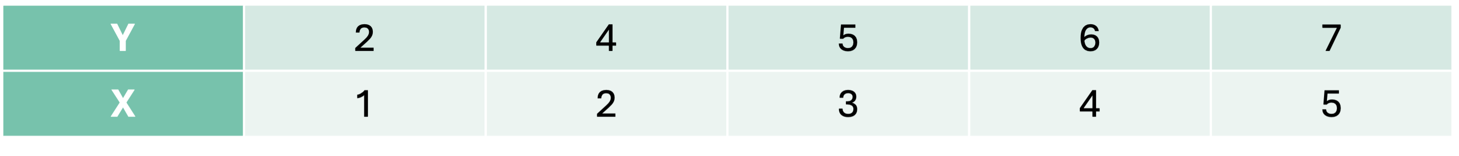{fig-align="center" width="6.5in"}We must split the data into 2 pieces based on the values of *X*. Here are all of the possible splits: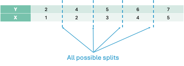{fig-align="center" width="6.5in"}Let's split the data in the first split point on the left hand side - an *X* value of 1.5. That would mean we have two groups - A and B.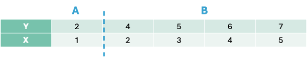{fig-align="center" width="6.5in"}The predictions from group A would be the average of the values of our target variable *y* from group A, $\hat{y} = 2$. The predictions of group B would be the average of *y* from group B, $\hat{y} = 5.5$.## SplittingThe main question is how we choose the best split. Splitting is done based on some condition. The **classification and regression tree (CART)** approach to decision trees uses mean square error (MSE) to decide the best split for continuous target variables and measurements of purity like Gini or entropy for classification target variables. The **chi-square automatic interaction detector (CHAID)** approach to decision trees uses $\chi^2$ tests and p-values to determine the best split.Let's continue the above example with the CART approach to decision trees. We will make the best split based on MSE. We want a split that will minimize the MSE for our predictions. Since we have the predictions for the first split above, let's calculate the MSE for each group:$$MSE_A = \frac{(2-2)^2}{1} = 0$$$$MSE_B = \frac{(4-5.5)^2 + (5-5.5)^2 + (6-5.5)^2 + (7-5.5)^2}{4} = 1.25$$Now, let's combine this into the overall MSE:$$MSE_{1.5} = 0.2 \times 0 + 0.8 \times 1.25 = 1$$Now let's move the split to the next possible location, 2.5: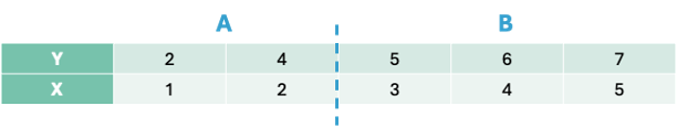{fig-align="center" width="6.5in"}Now our predictions for group A and B are $3$ and $6$ respectively. Let's again calculate the MSE for each group and the overall MSE for the split at 2.5:$$MSE_A = \frac{(2-3)^2 + (4-3)^2}{2} = 1$$$$MSE_B = \frac{(5-6)^2 + (6-6)^2 + (7-6)^2}{3} = 0.67$$$$MSE_{2.5} = 0.4 \times 1 + 0.6 \times 0.67 = 0.8$$This split has a lower overall MSE than the first split. In fact, if we were to continue this process for every split we would see that this split is the best of all possible binary splits.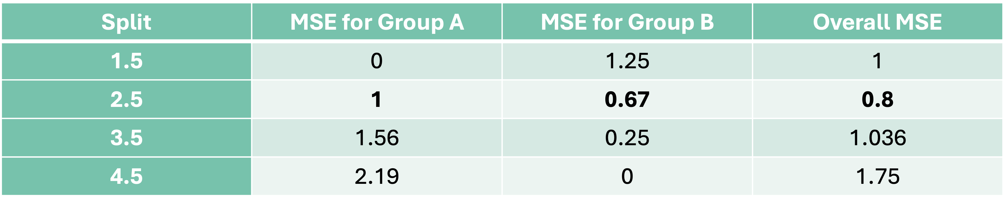{fig-align="center" width="8in"}Now we have our best decision tree model if we were to limit ourselves to splitting our data only once. Since our predictions are just the average of each group, we have a step function for our model as we can see below:```{python}#| echo: false#| warning: false#| error: false#| message: falseimport numpy as npimport matplotlib.pyplot as pltfrom sklearn.tree import DecisionTreeRegressor, plot_tree# 1. Simple 1D regression datasetX_little = np.array([[1], [2], [3], [4], [5]])y_little = np.array([2, 4, 5, 6, 7])# 2. Fit regression tree with max_depth=1 (only one split)reg = DecisionTreeRegressor(max_depth=1)reg.fit(X_little, y_little)# 3. Predict across a smooth range for visualizationx_vis = np.linspace(0.5, 5.5, 100).reshape(-1, 1)y_vis = reg.predict(x_vis)# 4. Plot the original points and predictionplt.figure(figsize=(10, 6))plt.scatter(X_little, y_little, color='black', label='Original data')plt.plot(x_vis, y_vis, color='red', label='Decision tree prediction', linewidth=2)plt.axvline(reg.tree_.threshold[0], color='blue', linestyle='--', label=f"Split at x = {reg.tree_.threshold[0]:.2f}")plt.title("Decision Tree Regressor (Depth=1) - Visualizing First Split")plt.xlabel("Feature X")plt.ylabel("Target y")plt.legend()plt.grid(True)plt.show()# 5. Print internal tree infoprint("Split Threshold:", reg.tree_.threshold[0])print("Left Node Prediction:", reg.tree_.value[reg.tree_.children_left[0]])print("Right Node Prediction:", reg.tree_.value[reg.tree_.children_right[0]])```Let's see how to build a simple CART decision tree in each software!::: {.panel-tabset .nav-pills}## PythonBuilding a CART decision tree in Python is rather simple. First, let's create the same dataset that we have been working with above by creating two arrays with the `numpy``array` function. Next, we just need the `DecisionTreeRegressor` function from the `sklearn.tree` package. We will set the `max_depth` option to 1 so that we will only find one split. Lastly, we just put the data arrays into the `fit` function and we have our model.```{python}#| warning: false#| error: false#| message: falseimport numpy as npimport matplotlib.pyplot as pltfrom sklearn.tree import DecisionTreeRegressor# Simple regression datasetX_little = np.array([[1], [2], [3], [4], [5]])y_little = np.array([2, 4, 5, 6, 7])# Fit regression tree with max_depth = 1 (only one split)model = DecisionTreeRegressor(max_depth =1)model.fit(X_little, y_little)```Unlike a linear regression, a decision tree's output is much more visual in nature. To do view the decision tree we can use the `plot_tree` function from the `sklearn.tree` package. The input to the `plot_tree` function is the decision tree model object from above. Most of the options are aesthetic in nature. However, the `feature_names` option is useful to see the actual variable names and the `proportion` option is used to show the proportion of the data in each node instead of raw counts.```{python}#| warning: false#| error: false#| message: falseimport matplotlib.pyplot as pltfrom sklearn.tree import plot_treeplt.figure(figsize = (12, 6))plot_tree( model, filled =True, feature_names = ["X"], rounded =True, proportion =True, precision =2, fontsize =12,)plt.title("Decision Tree Regressor Structure (max_depth=1)")plt.show()```From the above figure of the decision tree we can see the same structure and calculations we did by hand. The split is listed right at the top with the *X* variable optimally split at 2.5. In each piece we see the squared error on each side of the split, the percentage of observations in that split, and the predicted value in that piece of the split as well. Notice how the squared error, percentage of observations, and predicted values are exactly as calculated above.## RBuilding a CART decision tree in R is rather simple. First, let's create the same dataset that we have been working with above by creating a data frame with the `data.frame` function and a vector with a `c` function. Next, we just need the `rpart` function from the `rpart` package. We will set the `max_depth` option to 1 so that we will only find one split. Lastly, we just put the data into the `rpart` function using the typical formula framework. The `method = "anova"` option specifies that we will use MSE as our split decider. The `cp`, `minsplit`, and `minbucket` options were set to their smallest values since our toy example only had 5 observations.```{r}#| warning: false#| error: false#| message: falselibrary(rpart)X_little <-data.frame(x =c(1, 2, 3, 4, 5))y_little <-c(2, 4, 5, 6, 7)# Fit regression tree with maxdepth = 1 (only one split)model <-rpart(y_little ~ x, data = X_little, method ="anova", # "anova" is used for regressioncontrol =rpart.control(maxdepth =1, cp =0, minsplit =1, minbucket =1))# Print summary of the modelprint(model)```Unlike a linear regression, a decision tree's output is much more visual in nature. To do view the decision tree we can use the `rpart.plot` function from the `rpart.plot` package. The input to the `rpart.plot` function is the decision tree model object from above. Most of the options are aesthetic in nature.```{r}#| warning: false#| error: false#| message: falselibrary(rpart.plot)# Plot the decision treerpart.plot( model,type =2, extra =101, under =TRUE, faclen =0, fallen.leaves =TRUE,main ="Decision Tree Regressor Structure (max_depth = 1)",roundint =FALSE, digits =2, box.palette ="GnBu")```From the above figure of the decision tree we can see the same structure and calculations we did by hand. The split is listed right at the top with the *X* variable optimally split at 2.5. In each piece we see the percentage of observations in that split and the predicted value in that piece of the split as well. Notice how the percentage of observations and predicted values are exactly as calculated above.:::The exact same process would occur if we wanted to go 2 levels deep into our decision tree. Each piece of the decision tree would have the same process to see if additional splits within each of group A or group B would help improve the model's MSE. The predictions for a 2 level decision tree would be a more complicated step function as seen below:```{python}#| echo: false#| warning: false#| error: false#| message: falseimport numpy as npimport matplotlib.pyplot as pltfrom sklearn.tree import DecisionTreeRegressor, plot_tree# DataX_little = np.array([[1], [2], [3], [4], [5]])y_little = np.array([2, 4, 5, 6, 7])# Train regression tree with depth=2reg = DecisionTreeRegressor(max_depth=2, random_state=42)reg.fit(X_little, y_little)# Predictions for smooth plottingx_vis = np.linspace(0.5, 5.5, 500).reshape(-1, 1)y_vis = reg.predict(x_vis)import matplotlib.lines as mlinesplt.figure(figsize=(10, 6))plt.scatter(X_little, y_little, color='black', label='Training data')plt.plot(x_vis, y_vis, color='red', label='Tree prediction', linewidth=2)# Plot split lines without individual labelsthresholds = reg.tree_.thresholdfor t in thresholds:if t !=-2: plt.axvline(x=t, color='blue', linestyle='--')# Custom legend entry for all splitssplit_line = mlines.Line2D([], [], color='blue', linestyle='--', label='Splits')plt.legend(handles=[plt.Line2D([], [], color='red', linewidth=2, label='Tree prediction'), plt.Line2D([], [], marker='o', color='black', linestyle='', label='Training data'), split_line], loc='best')plt.title("Decision Tree Regressor (Depth=2) - Visualizing Splits")plt.xlabel("Feature X")plt.ylabel("Target y")plt.grid(True)plt.show()```Let's see how to do this in each software!::: {.panel-tabset .nav-pills}## PythonAdjusting the code to a 2 level decision tree in Python is just an adjustment to the `max_depth` option.```{python}#| warning: false#| error: false#| message: falseimport numpy as npimport matplotlib.pyplot as pltfrom sklearn.tree import DecisionTreeRegressor# Simple regression datasetX_little = np.array([[1], [2], [3], [4], [5]])y_little = np.array([2, 4, 5, 6, 7])# Fit regression tree with max_depth = 2 (only two splits)model = DecisionTreeRegressor(max_depth =2)model.fit(X, y)``````{python}#| warning: false#| error: false#| message: falseimport matplotlib.pyplot as pltfrom sklearn.tree import plot_treeplt.figure(figsize = (12, 6))plot_tree( reg, filled =True, feature_names = ["X"], rounded =True, proportion =True, precision =2, fontsize =12,)plt.title("Decision Tree Regressor Structure (max_depth=2)")plt.show()```The top node of the decision tree is referred to commonly as the **root node**. The very bottom nodes are sometimes called **leaves** or **terminal nodes**. Nodes can also be referred to as parent and children nodes. Children nodes are a level below their corresponding parent node.## RAdjusting the code to a 2 level decision tree in R is just an adjustment to the `max_depth` option.```{r}#| warning: false#| error: false#| message: falselibrary(rpart)X_little <-data.frame(x =c(1, 2, 3, 4, 5))y_little <-c(2, 4, 5, 6, 7)# Fit regression tree with maxdepth = 1 (only one split)model <-rpart(y_little ~ x, data = X_little, method ="anova", # "anova" is used for regressioncontrol =rpart.control(maxdepth =2, cp =0, minsplit =1, minbucket =1))# Print summary of the modelprint(model)``````{r}#| warning: false#| error: false#| message: falselibrary(rpart.plot)# Plot the decision treerpart.plot( model,type =2, extra =101, under =TRUE, faclen =0, fallen.leaves =TRUE,main ="Decision Tree Regressor Structure (max_depth = 1)",roundint =FALSE, digits =2, box.palette ="GnBu")```The top node of the decision tree is referred to commonly as the **root node**. The very bottom nodes are sometimes called **leaves** or **terminal nodes**. Nodes can also be referred to as parent and children nodes. Children nodes are a level below their corresponding parent node.:::## AttributesOne of the major reasons why decision trees are such a popular algorithm is that they are interpretable. With a series of binary decisions, you can easily follow why a prediction is the way that it is. You can also see if that specific split increases or decreases a prediction. These binary decisions are also very easy to implement into a system that scores customers.The models of decision trees are also more complicated than one might realize from an initial look at them. Decision trees and the step functions they produce for predictions are not limited to linear associations. The prediction of each final split is just the average of all of the observations in that group. This means the pattern could easily be nonlinear and that wouldn't impact the predictions from the decision tree. Each decision tree is also full of interactions between variables. Since each subsequent split after the first split is within each group, that implies that different groups after a split could be impacted differently by different variables. For example, A categorical *X2* variable might be important to split values below 2.5 from the variable *X*, but not values above 2.5.That previous point about variable splits impacting the decisions of variable splits after them implies that decision trees are **greedy algorithms**. Greedy algorithms makes the locally optimal choice at each step with the hope that these local decisions lead to a globally optimal solution. However, the decision tree only picks the next best option and doesn't go back to reconsider the choice after looking at the next decision points. This means there is not a guarantee of an optimal solution.## Tuning / Optimizing Decision TreesWith multiple variables, every variable is evaluated at every split to find the "best" single split across all possible splits across all possible variables. This includes categorical variables that have been dummy coded and each dummy coded variable is evaluated separately.With all of these variables and possible splits we have to worry about over-fitting our data. To prevent over-fitting of our data there are some common factors in a CART decision tree we can tune:- **Max depth of tree** - how many split levels overall in the tree- **Minimum samples in split** - how many observations must be in a node to even try to split- **Minimum samples in leaf** - how many observations left over in a leaf for a split to happenWhen it comes to tuning machine learning models like decision trees there are **many** options for tuning. **Cross-validation** should be included in each of these approaches. Two of the most common tuning approaches are:- Grid search- Bayesian optimizationGrid search algorithms look at a fixed grid of values for each parameter you can tune - called hyperparameters. This means that **every possible** combination of values no matter is they are good or bad as it doesn't learn from previous results. This is good for small samples with limited number of variables as it can be time consuming.Bayesian optimization on the other hand is typically less computationally expensive as a grid search approach. The Bayesian optimization approach starts with random values for each hyperparameter you need to tune. It then fits a probabilistic model (a type of sequential model-based optimization) that "learns" the relationship between the parameters and performance. This process tries to estimate which hyperparameters are likely to produce good results and point it in the "correct" direction for values of hyperparameters. The next step in the optimization essentially "learns" from the previous combinations of hyperparameters. This approach is much more valuable for large samples with large numbers of variables.We will continue to use our Ames housing dataset where we are predicting the sale price of a home. Even with tree-based algorithms, we still need to take the same steps to clean our data and do initial variable screening with business logic, low variability, missingness, and single variable comparison to the target. Machine learning models don't protect you to a point where you can just throw in horrible data!Let's tune these models in each software!::: {.panel-tabset .nav-pills}## PythonIn Python we will build and tune decision trees with both a grid search and Bayesian optimization approach to compare.Let's start with the grid search approach. We will use the `GridSearchCV` and `KFold` functions from the `sklearn.model_selection` package. The first thing we do is define the range of values for the grid search across each of the hyperparameters we want to tune. We will tune the options `max_depth`, `min_samples_split`, and `min_samples_leaf` which correspond to the above hyperparameters commonly tuned in decision trees. The `GridSearchCV` function will basically rerun the `DecisionTreeRegressor` function with each unique combination of values defined in the grid of hyperparameters. The `list` and `range` functions help put in values for those options. The `KFold` function defines the cross-validation that we will use. We will use a 10-fold cross-validation. The `DecisionTreeRegressor` model object, the parameter grid object, and cross-validation object are all inputs in the `GridSearchCV` function. The last thing to define is the `scoring` option where we will specify that we want to optimize the MSE. Specifically in Python, we optimize the negative MSE because it is a maximization algorithm instead of a minimization one.Once the grid search object is defined we just use the `fit` function along with our data to optimize the model. The `best_params_` function gives us the optimal combination of hyperparameters.```{python}#| warning: false#| error: false#| message: falsefrom sklearn.model_selection import GridSearchCV, KFold# Define parameter gridparam_grid = {'max_depth': list(range(2, 21)),'min_samples_split': list(range(2, 21)),'min_samples_leaf': list(range(1, 11))}cv = KFold(n_splits =10, shuffle =True, random_state =1234)# Initialize regressordt = DecisionTreeRegressor(random_state =1234)# Grid search with cross-validationgrid_search_reg = GridSearchCV(dt, param_grid = param_grid, cv = cv, scoring='neg_mean_squared_error')grid_search_reg.fit(X_reduced, y)# Best estimator and scoreprint("Best Regressor Params:", grid_search_reg.best_params_)```The best parameters according to the grid search are a max depth of 6, minimum samples per split of 16, and minimum samples per leaf at 2.Let's now build with Bayesian optimization. This involves slightly more complicated coding. First we must define our objective function where we similarly define our grid that we want to define. We will use the same hyperparameter values. We will still use the same `DecisionTreeRegressor` function as our grid search as well as the same `Kfold` function. The main differences come with the `create_study` function. This sets up the parameters previously defined with the objective. The `direction` option is used to tell the Bayesian optimization whether to maximize or minimize the outcome. The `sampler` option is where we control the seeding to make the optimization replicable. Inside of the `sampler` option we put in the `samplers.TPESampler` function with the seed set. Lastly, we use the `optimize` function with the defined objective on the `create_study` object. The `best_params` function gives us the optimal parameters from the Bayesian optimization.```{python}#| warning: false#| error: false#| message: falseimport optunafrom sklearn.tree import DecisionTreeRegressorfrom sklearn.model_selection import cross_val_score, train_test_splitfrom sklearn.metrics import mean_squared_error# Define the Optuna objective functiondef objective(trial): max_depth = trial.suggest_int("max_depth", 2, 20) min_samples_split = trial.suggest_int("min_samples_split", 2, 20) min_samples_leaf = trial.suggest_int("min_samples_leaf", 1, 10) dt = DecisionTreeRegressor( max_depth=max_depth, min_samples_split=min_samples_split, min_samples_leaf=min_samples_leaf, random_state=1234 )# Use negative MSE (Optuna tries to maximize the return value) cv = KFold(n_splits =10, shuffle =True, random_state =1234) score = cross_val_score(dt, X_reduced, y, cv=cv, scoring="neg_mean_squared_error")return score.mean() # This is negative MSE# Run Optuna studysampler = optuna.samplers.TPESampler(seed=1234)study = optuna.create_study(direction="maximize", sampler=sampler) # Because we're maximizing negative MSEstudy.optimize(objective, n_trials=50)# Resultsprint("Best Parameters:", study.best_params)```The best parameters according to the grid search are a max depth of 6, minimum samples per split of 19, and minimum samples per leaf at 2. This was calculated in a fraction of the time of the grid search.Let's build our optimized decision tree on our training dataset using these last parameter values given to us by the Bayesian optimization.```{python}#| warning: false#| error: false#| message: falsedt_ames = DecisionTreeRegressor(random_state =1234, max_depth =6, min_samples_split =19, min_samples_leaf =2)dt_ames.fit(X_reduced, y)# Visualizeplt.figure(figsize = (12, 6))plot_tree(dt_ames, feature_names = X_reduced.columns, filled =True, max_depth =2)plt.title("Decision Tree Regressor - Ames Housing Dataset")plt.show()```The tree plot above looks at the first two splits for our decision tree algorithm. The first split is on the overall quality of the home. The second split depends on the first split. If the overall quality of the home is high, then it looks at the square footage of the second floor. However, if the overall quality of the home is below 7.5 then it again splits on overall quality before looking at overall square footage.## RIn R we will build and tune decision trees with both a grid search and Bayesian optimization approach to compare.Let's start with the grid search approach. We will use the `train` and `trainControl` functions from the `caret` package. The first thing we do is define the range of values for the grid search across each of the hyperparameters we want to tune. In Python we have more control over the different tuning parameters we want in the decision tree as compared to R. With the `rpart` option inside of the `train` function we are only able to tune the `cp` option. The `cp` option controls the complexity parameter which corresponds to how much improvement we have to see in making a split. For example, a value of 0.01 would imply we need at least a 1% improvement for a split to occur. The `train` function will basically rerun the `rpart` function with each unique combination of values defined in the grid of hyperparameters. The `expand.grid` and `seq` functions help put in values for those options. The `trainControl` function defines the cross-validation that we will use. We will use a 10-fold cross-validation. The data, tuning grid, and cross-validation are all inputs to the `train` function. The last thing to define is the `metric` option where we will specify that we want to optimize the RMSE.The `bestTune` element of the tuned model gives us the optimal combination of hyperparameters.```{r}#| warning: false#| error: false#| message: falselibrary(caret)library(rpart)data <-data.frame(X_reduced, y = y)# Define the parameter gridgrid <-expand.grid(cp =seq(0.001, 0.05, by =0.001))# Define cross-validation folds (10-fold CV, shuffled)set.seed(1234)train_control <-trainControl(method ="cv", number =10)# Train the model using grid searchgrid_search_reg <-train( y ~ ., data = data,method ="rpart",trControl = train_control,tuneGrid = grid,metric ="RMSE")# Print best parametersprint(grid_search_reg$bestTune)```The best parameters according to the grid search are a complexity parameter of 0.001.Let's now build with Bayesian optimization. This involves slightly more complicated coding. First we must define our objective function where we similarly define our grid that we want to define. We will use the same hyperparameter values. We will still use the same `rpart` function as our grid search. The main differences come with the `bayesOpt` function. This sets up the parameters previously defined with the objective. The input to the `bayesOpt` function are all of the pieces we previously defined. The `bounds` option defines the specific values of the parameters we are tuning. The `getBestPars` function gives us the optimal parameters from the Bayesian optimization.```{r}#| warning: false#| error: false#| message: falselibrary(rpart)library(ParBayesianOptimization)data <-data.frame(X_reduced, y = y)# Define scoring function for Bayesian optimizationscore_func <-function(maxdepth, minsplit, minbucket) {# Ensure parameters are integers maxdepth <-round(maxdepth) minsplit <-round(minsplit) minbucket <-round(minbucket)# Train rpart with internal cross-validation model <-rpart( y ~ ., data = data,method ="anova",control =rpart.control(maxdepth = maxdepth,minsplit = minsplit,minbucket = minbucket,cp =0, # disable pruning, we tune maxdepthxval =10# 10-fold CV ) ) best_cp_row <-which.min(model$cptable[,"xerror"]) cv_error <- model$cptable[best_cp_row, "xerror"]# ParBayesianOptimization maximizes Score, so return negative RMSElist(Score =-cv_error)}# Define bounds for hyperparametersbounds <-list(maxdepth =c(2L, 20L),minsplit =c(2L, 20L),minbucket =c(1L, 10L))set.seed(1234)opt_results <-bayesOpt(FUN = score_func,bounds = bounds,initPoints =5, iters.n =50, # number of Bayesian optimization iterationsacq ="ucb", # acquisition functionverbose =0)# Best parametersbest_params <-getBestPars(opt_results)print(best_params)```The best parameters according to the grid search are a max depth of 11, minimum samples per split of 20, and minimum samples per leaf at 1.Let's build our optimized decision tree on our training dataset using these last parameter values given to us by the Bayesian optimization.```{r}#| warning: false#| error: false#| message: falsedt_ames <-rpart( y ~ .,data = data,method ="anova",control =rpart.control(maxdepth = best_params$maxdepth,minsplit = best_params$minsplit,minbucket = best_params$minbucket,cp =0 ))``````{r}#| warning: false#| error: false#| message: falselibrary(rpart.plot)# Plot the decision treerpart.plot( dt_ames,type =2, extra =101, under =TRUE, faclen =0, fallen.leaves =TRUE,main ="Decision Tree Regressor - Ames Housing Dataset",roundint =FALSE, digits =2, box.palette ="GnBu")```The tree plot above looks at our decision tree algorithm. The first split is on the overall quality of the home. The second split depends on the first split. If the overall quality of the home is high, then it looks at the square footage of the second floor. However, if the overall quality of the home is below 7.5 then it again splits on overall quality before looking at overall square footage.:::## Variable ImportanceMost machine learning models are **not** interpretable in the classical sense - as one predictor variable increases, the target variable tends to \_\_\_. This is because the relationships are not linear. The relationships are more complicated than a linear relationship, so the interpretations are as well. Decision trees, however, are still **interpretable** based on the decision framework they are built with.Although decision trees have an interpretable framework, we don't have p-values like we do in statistical regression modeling to help us understand variable importance. **Variable importance** is a way of telling which variables "mean more" to the model than other variables.In decision trees, the metric for variable importance is the MDI - **mean decrease in impurity**. Impurity has a different meaning depending on the type of target variable. In regression based trees with continuous target variables, the impurity metric is typically the variance of the residuals which is calculated by MSE. For classification based trees with a categorical target variable, the impurity metric is typically the Gini metric.The MSE calculation has been used many times before in this code deck, however, the Gini impurity metric is new. Let's look at its calculation:$$Gini = 1 - \sum_{i=1}^C p_i^2$$The calculation is quite simple. It calculates the proportion of each class in the target variable for the node and sums them together. This measure of impurity is a measure of **disorder** so we want lower values. Lower Gini impurity implies that the child nodes are "purer."Every time a feature is used to split a node, the software measures how much that split reduces the impurity. These reductions are accumulated across all trees for each feature (variable). These reductions are then normalized to sum to 1. The one problem with this approach is that it tends to overemphasize variables with many unique values because there are more places to split the variable.Let's calculate variable importance in each software!::: {.panel-tabset .nav-pills}## PythonPython automatically calculates the variable importance for decision trees as it build them. All we have to do is call the `feature_importances_` function on our model object. We could just use the `print` function to then print out the importance numbers. We plot them using the `seaborn` package below after sorting the importance values with the `sort_values` function.```{python}#| warning: false#| error: false#| message: falseimport matplotlib.pyplot as pltimport seaborn as sns# Get feature importancesimportances = dt_ames.feature_importances_# Create a Series with feature names and their importance scores then sortfeature_importances = pd.Series(importances, index = X_reduced.columns)sorted_importances = feature_importances.sort_values(ascending =False)# Plotplt.figure(figsize=(8, len(sorted_importances) *0.3)) # dynamic heightsns.barplot(x=sorted_importances.values, y=sorted_importances.index)plt.title("Feature Importances from Decision Tree")plt.xlabel("Importance Score")plt.ylabel("Features")plt.tight_layout()plt.show()```As we can see from the plot above, The overall quality of the home is the dominant feature in terms of importance of predicting sales price. This is followed by total square footage of the living area, second floor square footage, and so on. Any variables that have an importance score of 0 were not used at all during the building of the decision tree.## RR automatically calculates the variable importance for decision trees as it build them. All we have to do is call the `variable.importance` element on our model object. We could just use the `print` function to then print out the importance numbers. We plot them using the `ggplot2` package below after sorting the importance values with the `order` function.```{r}#| warning: false#| error: false#| message: falselibrary(ggplot2)importances <- dt_ames$variable.importanceimportance_df <-data.frame(Feature =names(importances),Importance =as.numeric(importances))importance_df <- importance_df[order(importance_df$Importance, decreasing =TRUE), ]# Plotggplot(importance_df, aes(x = Importance, y =reorder(Feature, Importance))) +geom_bar(stat ="identity", fill ="steelblue") +labs(title ="Feature Importances from Decision Tree",x ="Importance Score",y ="Features") +theme_minimal(base_size =12)```:::## PredictionsModels are nothing but potentially complicated formulas or rules. Once we determine the optimal model, we can **score** any new observations we want with the equation.::: callout-tip## ScoringIt's the process of applying a fitted model to input data to generate outputs like predicted values, probabilities, classifications, or scores.:::Scoring data **does not** mean that we are re-running the model/algorithm on this new data. It just means that we are asking the model for predictions on this new data - plugging the new data into the equation and recording the output. This means that our data must be in the same format as the data put into the model. Therefore, if you created any new variables, made any variable transformations, or imputed missing values, the same process must be taken with the new data you are about to score.For this problem we will score our test dataset that we have previously set aside as we were building our model. The test dataset is for comparing final models and reporting final model metrics. Make sure that you do **NOT** go back and rebuild your model after you score the test dataset. This would no longer make the test dataset an honest assessment of how good your model is actually doing. That also means that we should **NOT** just build hundreds of iterations of our same model to compare to the test dataset. That would essentially be doing the same thing as going back and rebuilding the model as you would be letting the test dataset decide on your final model.Let's score our data in each software!::: {.panel-tabset .nav-pills}## PythonWithout going into all of the same detail as before, the following code transforms the test dataset we originally created in the same way that we did for the training dataset by dropping necessary variables, making missing value imputations, and getting our same data objects.```{python}#| warning: false#| error: false#| message: falsepredictors_test = test.drop(columns=['SalePrice'])ames_dummied = pd.get_dummies(ames, drop_first=True)test_ids = test.indextest_dummied = ames_dummied.loc[test_ids]predictors_test = test_dummied.astype(float)predictors_test = predictors_test.drop(['GarageType_Missing', 'GarageQual_Missing','GarageCond_Missing'], axis=1)# Impute Missing for Continuous Variablesnum_cols = predictors_test.select_dtypes(include='number').columnsfor col in num_cols:if predictors_test[col].isnull().any(): predictors_test[f'{col}_was_missing'] = predictors_test[col].isnull().astype(int)# Impute with median median = predictors_test[col].median() predictors_test[col] = predictors_test[col].fillna(median)X_test = predictors_testy_test = test['SalePrice']y_test_log = np.log(test['SalePrice'])# Subset the DataFrame to selected featuresX_test_selected = X_test[selected_features].copy()```Now that our data is ready for scoring we can use the `predict` function on our model object we created with our decision tree. The only input to the `predict` function is the dataset we prepared for scoring.From the `sklearn.metrics` package we have a variety of model metric functions. We will use the `mean_absolute_error` (MAE) and `mean_absolute_percentage_error` (MAPE) metrics like the ones we described in the section on Model Building.```{python}#| warning: false#| error: false#| message: falsefrom sklearn.metrics import mean_absolute_errorfrom sklearn.metrics import mean_absolute_percentage_errorpredictions = dt_ames.predict(X_reduced)dt_pred = dt_ames.predict(X_test_selected)mae = mean_absolute_error(y_test, dt_pred)mape = mean_absolute_percentage_error(y_test, dt_pred)print(f"MAE: {mae:.2f}")print(f"MAPE: {mape:.2%}")```From the above output we can see that the linear regression model still beats thisd newly added decision tree.| Model | MAE | MAPE ||:-----------------:|:-----------:|:------:|| Linear Regression | \$18,160.24 | 11.36% || Ridge Regression | \$19.572.19 | 12.25% || GAM | \$18,154.31 | 11.40% || Decision Tree | \$25,422.52 | 16.01% |## RTo make sure that we are using the same test dataset between Python and R we will import our Python dataset here into R. There are a few variables that need to be renamed with the `names` function to work best in R.```{r}#| warning: false#| error: false#| message: falsey_test <- py$y_testX_test_selected <- py$X_test_selectednames(X_test_selected)[names(X_test_selected) =="1stFlrSF"] <-"FirstFlrSF"names(X_test_selected)[names(X_test_selected) =="2ndFlrSF"] <-"SecondFlrSF"names(X_test_selected)[names(X_test_selected) =="3SsnPorch"] <-"ThreeStoryPorch"```Now that our data is ready for scoring we can use the `predict` function on our model object we created with our decision tree. The only input to the `predict` function is the dataset we prepared for scoring with the `newdata` option.From the `Metrics` package we have a variety of model metric functions. We will use the `mae` (mean absolute error) and `mape` (mean absolute percentage error) metrics like the ones we described in the section on Model Building.```{r}#| warning: false#| error: false#| message: falselibrary(Metrics)predictions <-predict(dt_ames, newdata = X_reduced)dt_pred <-predict(dt_ames, newdata = X_test_selected)mae <-mae(y_test, dt_pred)mape <-mape(y_test, dt_pred)cat(sprintf("MAE: %.2f\n", mae))cat(sprintf("MAPE: %.2f%%\n", mape *100))```From the above output we can see that the linear regression model still beats this newly added decision tree.| Model | MAE | MAPE ||:-----------------:|:-----------:|:------:|| Linear Regression | \$18,160.24 | 11.36% || Ridge Regression | \$22,040.76 | 13.37% || GAM | \$19,479.79 | 12.23% || Decision Tree | \$22,934.49 | 13.92% |:::## SummaryIn summary, decision tree models are interpretable, decision based framework models. Some of the advantages of using decision trees:- Computationally fast- Still interpretable due to decision framework output- Easy to implement- Variable importance providedThere are some disadvantages though:- Typically, not as predictive as more advanced models- Greedy algorithm means every decision is completely based on the previous decision- Bias towards features with more levels# BaggingBefore understanding the concept of **bagging**, we need to know what a **bootstrap sample** is. A Bootstrap sample is a random sample of your data *with replacement* that are the same size as your original data set. By random chance, some of the observations will not be sampled. These observations are called **out-of-bag** observations. Three example bootstrap samples of 10 observations labelled 1 through 10 are listed below:{fig-align="center" width="7in"}Mathematically, a bootstrap sample will contain approximately 63% of the observations in the data set. The sample size of the bootstrap sample is the same as the original data set, just some observations are repeated. Bootstrap samples are used in simulation to help develop confidence intervals of complicated forecasting techniques. Bootstrap samples are also used to ensemble models using different training data sets - called **bagging**.**B**ootstrap **agg**regat**ing** (bagging) is where you take *k* bootstrap samples and create a model using each of the bootstrap samples as the training data set. This will build *k* different models. We will ensemble these *k* different models together.Let's work through an example to see the potential value. The following 10 observations have the values of X and Y shown in the following table:{fig-align="center" width="8in"}We will build a decision stump (a decision tree with only one split). From building a decision stump, the best accuracy is obtained by making the split at either 3.5 or 7.5. Either of these splits would lead to an accuracy of predicting Y at 70%. For example, let's use the split at 3.5. That would mean we think everything above 3.5 is a 0 and everything below 3.5 is a 1. We would get observations 1, 2, and 3 all correct. However, since everything above 3.5 is considered a 0, we would only get observations 4, 5, 6, and 7 correct on that piece - missing observations 8, 9, and 10.{fig-align="center" width="8in"}To try and make this prediction better we will do the following:1. Take 10 bootstrap samples2. Build a decision stump for each3. Aggregate these rules into a voting ensemble4. Test the performance of the voting ensemble on the whole datasetThe following is the 10 bootstrap samples with their optimal splits. Remember, these bootstrap samples will not contain all of the observations in the original data set.{fig-align="center" width="8in"}{fig-align="center" width="8in"}Some of these samples contain only one value of the target variable and so the predictions are the same for that bootstrap sample. However, we will use the optimal cut-offs from each of those samples to predict 1's and 0's for the *original* data set as shown in the table below:{fig-align="center" width="8in"}The table above has one row for each of the predictions from the 10 bootstrap samples. We can average these predictions of 1's and 0's together for each observation to get the average row near the bottom.Let's take a cut-off of 0.25 from our average values from the 1 and 0 predictions from each bootstrap sample. That would mean anything above 0.25 in the average row would be predicted as a 1 while everything below would be predicted as a 0. Based on those predictions (the Pred. row above) we get a perfect prediction compared to the true values of Y from our original data set.In summary, bagging improves generalization error on models with high variance (simple tree-based models for example). If base classifier is stable (not suffering from high variance), then bagging can actually make predictions worse! Bagging does not focus on particular observations in the training data set (unlike boosting which is covered below).# Random Forests**Random forests** are ensembles of decision trees (similar to the bagging example from above). Ensembles of decision trees work best when they find different patterns in the data. However, bagging tends to create trees that pick up the same pattern.Random forests get around this correlation between trees by not only using bootstrapped samples, but also uses subsets of variables for each split and unpruned decision trees. For these unpruned trees, with a classification target it goes all the way until each unique observation is left in its own leaf. With regression trees the unpruned trees will continue until 5 observations are left per leaf. The results from all of these trees are ensembled together into one voting system. There are many choices of parameters to tune:1. Number of trees in the ensemble2. Number of variables for each split3. Depth of the tree (defaults to unpruned)## Building Random ForestLet's see random forests in each software!::: {.panel-tabset .nav-pills}## PythonLet's build a random forest with our Ames housing data set. We will use the `RandomForestRegressor` function from the `sklearn.ensemble` package. Similar to other Python functions we have used, we need the training predictor variables in one object and the target variable in another. The option to define how many decision trees are in the ensemble is `n_estimators`.```{python}#| warning: false#| error: false#| message: falsefrom sklearn.ensemble import RandomForestRegressorrf_ames = RandomForestRegressor(n_estimators =100, random_state =1234, oob_score =True)rf_ames.fit(X_reduced, y)```The `random_state` option helps set the seed for the function to make the results repeatable. The `oob_score = True` option calculates the out-of-bag score for the model chosen for comparisons to other models of different sizes. For continuous targets it provides the $R^2$ metric. For categorical targets this option provides the AUC. Let's view that out-of-bag score with call of the `oos_score_` element from the model object.```{python}#| warning: false#| error: false#| message: falserf_ames.oob_score_```## RLet's build a random forest with our Ames housing data set. We will use the `randomForest` function from the `randomForest` package. Similar to other R functions we have used, we need the training predictor variables in one object and the target variable in another. The option to define how many decision trees are in the ensemble is `ntree`.```{r}#| warning: false#| error: false#| message: falselibrary(randomForest)set.seed(1234)# Fit random forestrf_ames <-randomForest(x = X_reduced,y = y,ntree =500, importance =TRUE, keep.inbag =TRUE)# Check OOB R^2print(rf_ames)```The `set.seed` option helps set the seed for the function to make the results repeatable. The `importance = True` option calculates the variable importance for the variables in the random forest. With the `print` function we can see the $R^2$ of the model as the percentage of the variance explained.:::## Tuning / Optimizing Random ForestsThere are a few things we can tune with a random forest. One is the number of trees used to build the model. Another thing to tune is the number of variables considered for each split - called **mtry**. By default, $mtry = \sqrt{p}$, with $p$ being the number of total variables. We can use cross-validation to tune these values. Just like with decision trees, we can use either a grid search approach or Bayesian optimization.Let's see how to do this in each software!::: {.panel-tabset .nav-pills}## PythonIn Python we will build and tune random forests with both a grid search and Bayesian optimization approach to compare.Let's start with the grid search approach. In Python we can use the `GridSearchCV` function from the `sklearn.model_selection` package. In this function we need to define a grid to search across for the parameters to tune. Here are three common parameters to tune in the `RandomForestRegressor` function - `max_depth` which controls the depth of the trees, `max_features` which is *mtry*, and `n_estimators` which is the number of trees. The `GridSearchCV` function will basically rerun the `RandomForestRegressor` function with each unique combination of values defined in the grid of hyperparameters. The `list` and `range` functions help put in values for those options. The `KFold` function defines the cross-validation that we will use. We will use a 10-fold cross-validation. The `RandomForestRegressor` model object, the parameter grid object, and cross-validation object are all inputs in the `GridSearchCV` function. The last thing to define is the `scoring` option where we will specify that we want to optimize the MSE. Specifically in Python, we optimize the negative MSE because it is a maximization algorithm instead of a minimization one.Once the grid search object is defined we just use the `fit` function along with our data to optimize the model. The `best_params_` function gives us the optimal combination of hyperparameters.```{python}#| warning: false#| error: false#| message: falsefrom sklearn.model_selection import GridSearchCV, KFoldparam_grid = {'max_depth': [None, 10, 20, 30],'max_features': [3, 4, 5, 6, 7],'n_estimators': [100, 200, 300, 400, 500, 600, 700, 800]}cv = KFold(n_splits =10, shuffle =True, random_state =1234)rf = RandomForestRegressor(random_state =1234)grid_search = GridSearchCV(estimator = rf, param_grid = param_grid, cv = cv, scoring ='neg_mean_squared_error')grid_search.fit(X_reduced, y)grid_search.best_params_```The best parameters according to the grid search are a max depth of 20, maximum number of features at 5, and 200 trees.Let's now build with Bayesian optimization. This involves slightly more complicated coding. First we must define our objective function where we similarly define our grid that we want to define. We will use the same hyperparameter values. We will still use the same `RandomForestRegressor` function as our grid search as well as the same `Kfold` function. The main differences come with the `create_study` function. This sets up the parameters previously defined with the objective. The `direction` option is used to tell the Bayesian optimization whether to maximize or minimize the outcome. The `sampler` option is where we control the seeding to make the optimization replicable. Inside of the `sampler` option we put in the `samplers.TPESampler` function with the seed set. Lastly, we use the `optimize` function with the defined objective on the `create_study` object. The `best_params` function gives us the optimal parameters from the Bayesian optimization.```{python}#| warning: false#| error: false#| message: falseimport optunafrom sklearn.model_selection import cross_val_scoreimport numpy as np# Step 1: Define the objective using a lambda so you keep your code flatdef objective(trial):# Define search space (equivalent to your param_grid) max_depth = trial.suggest_categorical('max_depth', [None, 10, 20, 30]) max_features = trial.suggest_int('max_features', 3, 7) n_estimators = trial.suggest_int('n_estimators', 100, 800, step=100)# Create the model with suggested parameters rf = RandomForestRegressor( max_depth = max_depth, max_features = max_features, n_estimators = n_estimators, random_state =1234 )# 10-fold CV like your original cv = KFold(n_splits =10, shuffle =True, random_state =1234) scores = cross_val_score(rf, X_reduced, y, cv = cv, scoring ='neg_mean_squared_error') # or 'r2'return np.mean(scores)# Step 2: Run the optimizationsampler = optuna.samplers.TPESampler(seed=1234)study = optuna.create_study(direction="maximize", sampler=sampler) # 'minimize' for error metricsstudy.optimize(objective, n_trials =50, show_progress_bar =True)# Step 3: Get the best hyperparametersprint("Best parameters:", study.best_params)print("Best score:", study.best_value)```The best parameters according to the grid search are a max depth of 30, maximum number of features at 6, and 400 trees. This was calculated in a fraction of the time of the grid search.Let's build our optimized random forest on our training dataset using these last parameter values given to us by the Bayesian optimization.```{python}#| warning: false#| error: false#| message: falserf_ames = RandomForestRegressor(n_estimators =400, max_features =6, max_depth =30, random_state =1234, oob_score =True)rf_ames.fit(X_reduced, y)```## RIn R we will build and tune random forests with both a grid search and Bayesian optimization approach to compare.Let's start with the grid search approach. To start tuning our random forests in R we will look at the number of trees we would like. We will use the `plot` function to see how the number of trees increasing improves the MSE of the model.```{r}#| warning: false#| error: false#| message: falseplot(rf_ames, main ="Number of Trees Compared to MSE")```We can see from the plot above that the MSE of the whole training set seems to level off around 300 trees. Beyond that, adding more trees only increases the computation time, but not the predictive power of the model.We will use the `train` and `trainControl` functions from the `caret` package to finish the tuning. The first thing we do is define the range of values for the grid search across each of the hyperparameters we want to tune. In Python we have more control over the different tuning parameters we want in the random forest as compared to R. With the `rf` option inside of the `train` function we are only able to tune the `mtry` option. The `mtry` option controls the number of variables allowed for each split. The `train` function will basically rerun the random forest with each unique combination of values defined in the grid of hyperparameters. The `expand.grid` and `c` functions help put in values for those options. The `trainControl` function defines the cross-validation that we will use. We will use a 10-fold cross-validation. The data, tuning grid, and cross-validation are all inputs to the `train` function. The last thing to define is the `metric` option where we will specify that we want to optimize the RMSE.The `bestTune` element of the tuned model gives us the optimal combination of hyperparameters.```{r}#| warning: false#| error: false#| message: falselibrary(caret)library(randomForest)set.seed(1234)# 10-fold CVcv_control <-trainControl(method ="cv",number =10)# Grid over mtry onlytune_grid <-expand.grid(mtry =c(3, 4, 5, 6, 7))y <-as.numeric(y)# Train random forestrf_model <-train(x = X_reduced,y = y,method ="rf",metric ="RMSE",trControl = cv_control,tuneGrid = tune_grid,ntree =300, # fixed number of treesmaxnodes =30# optional: limit tree depth)# Best mtryprint(rf_model$bestTune)```The best parameters according to the grid search are an *mtry* parameter of 7.Let's now build with Bayesian optimization. This involves slightly more complicated coding. First we must define our objective function where we similarly define our grid that we want to define. We will use the same hyperparameter values. We will still use the same `train` function as our grid search. The main differences come with the `bayesOpt` function and the method now being `ranger`. This is a different functionality for building random forests compared to the `randomForest` function. With this functionality in a Bayesian optimization we have the ability to actually optimize the number of trees, *mtry*, and max depth of the trees. The input to the `bayesOpt` function are all of the pieces we previously defined. The `bounds` option defines the specific values of the parameters we are tuning. The `getBestPars` function gives us the optimal parameters from the Bayesian optimization.```{r}#| warning: false#| error: false#| message: falselibrary(caret)library(ranger)library(ParBayesianOptimization)set.seed(1234)y <-as.numeric(y)# Define the scoring function for Bayesian Optimizationrf_bayes_caret <-function(mtry, num.trees, max.depth) {# Convert parameters to integers mtry <-as.integer(mtry) num.trees <-as.integer(num.trees) max.depth <-ifelse(max.depth ==0, NULL, as.integer(max.depth))# Train using caret with 10-fold CV model <-train(x = X_reduced,y = y,method ="ranger",tuneGrid =data.frame(mtry = mtry, splitrule ="variance", min.node.size =5),trControl =trainControl(method ="cv", number =10),num.trees = num.trees,max.depth = max.depth,importance ="impurity" )# Return negative RMSE for maximization (like neg_mean_squared_error)list(Score =-min(model$results$RMSE))}# Define bounds for Bayesian Optimizationbounds <-list(mtry =c(3L, 7L),num.trees =c(100L, 800L),max.depth =c(0L, 30L) # 0 = unlimited depth)# Run Bayesian Optimizationopt_res <-bayesOpt(FUN = rf_bayes_caret,bounds = bounds,initPoints =5,iters.n =50,acq ="ei",verbose =0)# Best parametersbest_params <-getBestPars(opt_res)best_score <--opt_res$scoreSummary$Score[which.max(opt_res$scoreSummary$Score)]print(best_params)print(best_score)```The best parameters according to the grid search are a max depth of 19, maximum number of features at 7, and 800 trees. This was calculated in a fraction of the time of the grid search.Let's build our optimized random forest on our training dataset using these last parameter values given to us by the Bayesian optimization.```{r}#| warning: false#| error: false#| message: falselibrary(caret)library(ranger)# Extract best parametersbest_mtry <-as.integer(best_params$mtry)best_num_trees <-as.integer(best_params$num.trees)best_max_depth <-ifelse(best_params$max.depth ==0, NULL, as.integer(best_params$max.depth))# Train final model using the entire datasetfinal_rf <-train(x = X_reduced,y = y,method ="ranger",tuneGrid =data.frame(mtry = best_mtry, splitrule ="variance", min.node.size =5),trControl =trainControl(method ="none"), num.trees = best_num_trees,max.depth = best_max_depth,importance ="impurity")# The ranger model is insiderf_ames <- final_rf$finalModel```:::## Variable ImportanceMost machine learning models are **not** interpretable in the classical sense - as one predictor variable increases, the target variable tends to \_\_\_. This is because the relationships are not linear. The relationships are more complicated than a linear relationship, so the interpretations are as well. Random forests are an aggregation of many decision trees which makes this general interpretation difficult. We cannot view the tree like we can with a simple decision tree. Again, we will have to use our metrics for variable importance like we did with decision trees.Just like in decision trees, the metric for variable importance in random forests is the MDI - **mean decrease in impurity**. Impurity has a different meaning depending on the type of target variable. In regression based trees with continuous target variables, the impurity metric is typically the variance of the residuals which is calculated by MSE. For classification based trees with a categorical target variable, the impurity metric is typically the Gini metric.Every time a feature is used to split a node, the software measures how much that split reduces the impurity. These reductions are accumulated across all trees for each feature (variable). These reductions are then normalized to sum to 1. The one problem with this approach is that it tends to overemphasize variables with many unique values because there are more places to split the variable.Let's calculate variable importance in each software!::: {.panel-tabset .nav-pills}## PythonPython automatically calculates the variable importance for random forests as it build them. All we have to do is call the `feature_importances_` function on our model object. We could just use the `print` function to then print out the importance numbers. We plot them using the `seaborn` package below after sorting the importance values with the `sort_values` function.```{python}#| warning: false#| error: false#| message: falseimportances = rf_ames.feature_importances_feature_importances = pd.Series(importances, index=X_reduced.columns)sorted_importances = feature_importances.sort_values(ascending=False)plt.figure(figsize=(8, len(sorted_importances) *0.3))sns.barplot(x=sorted_importances.values, y=sorted_importances.index)plt.title("Feature Importances from Random Forest")plt.xlabel("Importance Score")plt.ylabel("Features")plt.tight_layout()plt.show()```As we can see from the plot above, The overall quality of the home and greater living area are the dominant features in terms of importance of predicting sales price. These are followed by the number of garage cars, the garage square footage, and so on. Any variables that have an importance score of 0 were not used at all during the building of the random forest.## RR automatically calculates the variable importance for random forests as it build them. All we have to do is call the `variable.importance` element on our model object. We could just use the `print` function to then print out the importance numbers. We plot them using the `ggplot2` package below after sorting the importance values with the `order` function.```{r}#| warning: false#| error: false#| message: falselibrary(ggplot2)library(dplyr)# Extract feature importances from a ranger random forestimportances <- rf_ames$variable.importance# Convert to a data frame and sortfeature_importances <-data.frame(Feature =names(importances),Importance = importances) %>%arrange(desc(Importance))# Plotggplot(feature_importances, aes(x = Importance, y =reorder(Feature, Importance))) +geom_bar(stat ="identity", fill ="steelblue") +labs(title ="Feature Importances from Random Forest",x ="Importance Score",y ="Features" ) +theme_minimal() +theme(plot.title =element_text(hjust =0.5),axis.text.y =element_text(size =10) )```As we can see from the plot above, The overall quality of the home is the dominant feature in terms of importance of predicting sales price. That is followed by the size fo the home, number of garage cars, the basement square footage, and so on. Any variables that have an importance score of 0 were not used at all during the building of the random forest.:::## Variable SelectionAnother thing to tune would be which variables to include in the random forest. By default, random forests use all the variables since they are averaged across all the trees used to build the model. There are a couple of ways to perform variable selection for random forests:- Many permutations of including/excluding variables- Compare variables to random variableThe first approach is rather straight forward but time consuming because you have to try and build models over and over again taking a variable out each time. The second approach is much easier to try. In that second approach we will create a completely random variable and put it in the model. We will then look at the variable importance of all the variables. The variables that are below the random variable should be considered for removal.Let's see this in each software!::: {.panel-tabset .nav-pills}## PythonTo create a random variable in Python we will first create a new data frame called `X_reduced_r` from a copy of our dataset using the `copy` function. We will then add a variable called *random* with the `random.normal` function from numpy.```{python}#| warning: false#| error: false#| message: falseimport numpy as npX_reduced_r = X_reduced.copy()X_reduced_r['random'] = np.random.normal(0, 1, X_reduced.shape[0])```We then build a random forest model in the same way we did previously and check the variable importance.```{python}#| warning: false#| error: false#| message: falserf_ames_r = RandomForestRegressor(n_estimators =400, max_features =6, max_depth =30, random_state =1234, oob_score =True)rf_ames_r.fit(X_reduced_r, y)# Name of the variable to highlighthighlight_feature ="random"# Get importancesimportances = rf_ames_r.feature_importances_feature_importances = pd.Series(importances, index=X_reduced_r.columns)sorted_importances = feature_importances.sort_values(ascending=False)# Define colors: use a different color for the highlighted featurecolors = ['orange'if feat == highlight_feature else'gray'for feat in sorted_importances.index]# Plotplt.figure(figsize=(8, len(sorted_importances) *0.3)) # dynamic heightsns.barplot(x=sorted_importances.values, y=sorted_importances.index, palette=colors)plt.title("Feature Importances from Random Forest")plt.xlabel("Importance Score")plt.ylabel("Features")plt.tight_layout()plt.show()```Based on the plot above there are 26 variables that fall below the variable importance of the random variable that could be considered for removal from the model.## RTo create a random variable in R we will just use the `rnorm` function with a mean of 0, standard deviation of 1 (both defaults) and a count of the number of observations in our training data.```{r}#| warning: false#| error: false#| message: falselibrary(dplyr)set.seed(1234)# Copy X_reduced and add a random featureX_reduced_r <- X_reducedX_reduced_r$random <-rnorm(nrow(X_reduced_r), mean =0, sd =1)```We then build a random forest model in the same way we did previously and check the variable importance.```{r}#| warning: false#| error: false#| message: falselibrary(ranger)library(ggplot2)# Train random forest with rangerrf_ames_r <-ranger(dependent.variable.name ="y",data =cbind(y = y, X_reduced_r),num.trees =400,mtry =6,max.depth =30,importance ="impurity",seed =1234)# Extract variable importancesimportances <- rf_ames_r$variable.importancefeature_importances <-data.frame(Feature =names(importances),Importance = importances) %>%arrange(desc(Importance))# Define highlight featurehighlight_feature <-"random"feature_importances$Color <-ifelse(feature_importances$Feature == highlight_feature, "orange", "gray")# Plotggplot(feature_importances, aes(x = Importance, y =reorder(Feature, Importance), fill = Color)) +geom_bar(stat ="identity") +scale_fill_identity() +labs(title ="Feature Importances from Random Forest",x ="Importance Score",y ="Features" ) +theme_minimal() +theme(plot.title =element_text(hjust =0.5),axis.text.y =element_text(size =10) )```Based on the plot above there are 25 variables that fall below the variable importance of the random variable that could be considered for removal from the model.:::## "Interpretability"Most machine learning models are **not** interpretable in the classical sense - as one predictor variable increases, the target variable tends to \_\_\_. This is because the relationships are not linear. The relationships are more complicated than a linear relationship, so the interpretations are as well. Similar to GAM's we can get a general idea of an overall pattern for a predictor variable compared to a target variable - **partial dependence plots**.These plots will be covered in much more detail in the final section of this code deck under Model Agnostic Interpretability.```{python}#| warning: false#| error: false#| message: false#| echo: falseimport matplotlib.pyplot as pltfrom sklearn.inspection import PartialDependenceDisplay# Plot for one or more featuresfeatures_to_plot = ['GrLivArea']PartialDependenceDisplay.from_estimator(rf_ames, X_reduced, features_to_plot, kind="average", percentiles=(0.0, 1.0))plt.tight_layout()plt.show()```This nonlinear and complex relationship between *GrLivArea* and *SalePrice* is similar to the plot we saw earlier with the GAMs. This shouldn't be too surprising. Both sets of algorithms are trying to relate these two variables together, just in different ways.## PredictionsModels are nothing but potentially complicated formulas or rules. Once we determine the optimal model, we can **score** any new observations we want with the equation.Scoring data **does not** mean that we are re-running the model/algorithm on this new data. It just means that we are asking the model for predictions on this new data - plugging the new data into the equation and recording the output. This means that our data must be in the same format as the data put into the model. Therefore, if you created any new variables, made any variable transformations, or imputed missing values, the same process must be taken with the new data you are about to score.For this problem we will score our test dataset that we have previously set aside as we were building our model. The test dataset is for comparing final models and reporting final model metrics. Make sure that you do **NOT** go back and rebuild your model after you score the test dataset. This would no longer make the test dataset an honest assessment of how good your model is actually doing. That also means that we should **NOT** just build hundreds of iterations of our same model to compare to the test dataset. That would essentially be doing the same thing as going back and rebuilding the model as you would be letting the test dataset decide on your final model.Let's score our data in each software!::: {.panel-tabset .nav-pills}## PythonNow that our data is ready for scoring based on the code for the decision tree model, we can use the `predict` function on our model object we created with our random forest. The only input to the `predict` function is the dataset we prepared for scoring.From the `sklearn.metrics` package we have a variety of model metric functions. We will use the `mean_absolute_error` (MAE) and `mean_absolute_percentage_error` (MAPE) metrics like the ones we described in the section on Model Building.```{python}#| warning: false#| error: false#| message: falsefrom sklearn.metrics import mean_absolute_errorfrom sklearn.metrics import mean_absolute_percentage_errorpredictions = rf_ames.predict(X_reduced)rf_pred = rf_ames.predict(X_test_selected)mae = mean_absolute_error(y_test, rf_pred)mape = mean_absolute_percentage_error(y_test, rf_pred)print(f"MAE: {mae:.2f}")print(f"MAPE: {mape:.2%}")```From the above output we can see that the linear regression model still beats a lot of the algorithms we've tried. However, the random forest is now the best performing model overall as it is the first model to beat the linear regression.| Model | MAE | MAPE ||:-----------------:|:-----------:|:------:|| Linear Regression | \$18,160.24 | 11.36% || Ridge Regression | \$19.572.19 | 12.25% || GAM | \$18,154.31 | 11.40% || Decision Tree | \$25,422.52 | 16.01% || Random Forest | \$16,974.22 | 10.90% |## RNow that our data is ready for scoring based on the code for the decision tree model, we can use the `predict` function on our model object we created with our random forest. The only input to the `predict` function is the dataset we prepared for scoring. We then just call the `predictions` element.From the `Metrics` package we have a variety of model metric functions. We will use the `mae` (mean absolute error) and `mape` (mean absolute percentage error) metrics like the ones we described in the section on Model Building.```{r}#| warning: false#| error: false#| message: falselibrary(Metrics)predictions <-predict(rf_ames, data = X_reduced)$predictionsrf_pred <-predict(rf_ames, data = X_test_selected)$predictionsmae <-mae(y_test, rf_pred)mape <-mape(y_test, rf_pred)cat(sprintf("MAE: %.2f\n", mae))cat(sprintf("MAPE: %.2f%%\n", mape *100))```From the above output we can see that the linear regression model still beats a lot of the algorithms we've tried. However, the random forest is now the best performing model overall as it is the first model to beat the linear regression.| Model | MAE | MAPE ||:-----------------:|:-----------:|:------:|| Linear Regression | \$18,160.24 | 11.36% || Ridge Regression | \$22,040.76 | 13.37% || GAM | \$19,479.79 | 12.23% || Decision Tree | \$22,934.49 | 13.92% || Random Forest | \$16,864.85 | 10.77% |:::## SummaryIn summary, random forest models are good models to use for prediction, but explanation becomes more difficult and complex. Some of the advantages of using random forests:- Computationally fast (handles thousands of variables)- Trees trained simultaneously- Accurate **classification** model- Variable importance available- Missing data is OKThere are some disadvantages though:- "Interpretability" is a little different than the classical sense- There are parameters that need to be tuned to make the model the best# BoostingBoosting is similar to bagging in the sense that we will draw a sample of observations from a data set with replacement. However, unlike bagging, observations are **not** sampled randomly. Boosting assigns weights to each training observation and uses the weight as a sampling distribution. Observations with higher weights are more likely to be drawn in the next sample. These weights are changed adaptively in each round. The weights for observations that are harder to classify are higher for the next sample - trying to increase chance of them being selected. We want these missed observations to have a higher chance of being in the next model to improve the chances of predicting those observations correctly the next time. An example of the difference in weights for a boosted sample as compared to a bagging sample is the following:{fig-align="center" width="8in"}With bagging we are only trying to create variability in the models by using training data set variation. The ensemble model is built **simultaneously**. However, in boosting, observations with higher sampling probability were harder to predict accurately. We want to improve the predictions from the model **sequentially**.Let's use the same example we used in bagging. The following 10 observations have the values of X and Y shown in the following table:{fig-align="center" width="8in"}We will build a decision stump (a decision tree with only one split). From building a decision stump, the best accuracy is obtained by making the split at either 3.5 or 7.5. Either of these splits would lead to an accuracy of predicting Y at 70%. For example, let's use the split at 3.5. That would mean we think everything above 3.5 is a 0 and everything below 3.5 is a 1. We would get observations 1, 2, and 3 all correct. However, since everything above 3.5 is considered a 0, we would only get observations 4, 5, 6, and 7 correct on that half - missing observations 8, 9, and 10.{fig-align="center" width="8in"}To try and make this prediction better we will do the following:1. Take 3 bootstrap samples2. Build a decision stump for each3. At each step we will adjust the weights based on the previous step's errorsThe following is the first 3 bootstrap samples with their optimal splits. Remember, these bootstrap samples will not contain all of the observations in the original data set.{fig-align="center" width="8in"}The first sample has the same weight for each observation. In that bootstrap sample the best split occurs at 7.5. However, when predicting the original observations, we would **incorrectly** predict observations 1, 2, and 3. Therefore, in the second sample we will overweight observations 1, 2, and 3 to help us predict those observations better (correct for the previous mistakes). In the second bootstrap sample we have observations 1, 2, and 3 over-represented by design. However, this leads to incorrect predictions in observations 4 through 7. This will lead to us over-weighting those observations as seen in the third row of the weights table. Observations 8, 9, and 10 have always been correctly predicted so their weight is the smallest, while the other observations have higher weights.The original boosted sample ensemble was called AdaBoost. Unlike bagging, boosted ensembles usually weight the votes of each classifier by a function of their accuracy. If the classifier gets the higher weighted observations wrong, it has a higher error rate. More accurate classifiers get a higher weight in the prediction. In simple terms, more accurate guesses are more important. We will not detail this algorithm here as there are more common advancements that have come since.# Gradient BoostingSome more recent algorithms are moving away from the direct boosting approach applied to bootstrap samples. However, the main idea of these algorithms is still rooted in the notion of finding where you made mistakes and trying to improve on those mistakes.One of the original algorithms to go with this approach is the **gradient boosted machine** (GBM). The idea behind the GBM is to build a simple model to predict the target (much like a decision tree or even decision stump):$$y = f_1(x) + \varepsilon_1 $$That simple model has an error of $\varepsilon_1$. The next step is to try to **predict that error** with another simple model:$$\varepsilon_1 = f_2(x) + \varepsilon_2$$This model has an error of $\varepsilon_2$. We can continue to add model after model, each one predicting the error (residuals) from the previous round:$$y = f_1(x) + f_2(x) + \cdots + f_k(x) + \varepsilon_k$$We will continue this process until there is a really small error which will lead to over-fitting. To protect against over-fitting, we will build in gradient boosting regularization through parameters to tune. One of those parameters to tune is $\eta$, which is the weight applied to the error models:$$y = f_1(x) + \eta \times f_2(x) + \eta \times f_3(x) + \cdots + \eta \times f_k(x) + \varepsilon_k$$Smaller values of $\eta$ lead to less over-fitting. Other things to tune include the number of trees to use in the prediction (more trees typically lead to more over-fitting), and other parameters added over the years - $\lambda$, $\gamma$, $L_2$, etc.Gradient boosting as defined above yields an additive ensemble model. There is no voting or averaging of individual models as the models are built sequentially, not simultaneously. The predictions from these models are added together to get the final prediction. One of the big keys to gradient boosting is using **weak learners**. Weak learners are simple models. Shallow decision / regression trees are the best. Each of these models would make poor predictions on their own, but the additive fashion of the ensemble provides really good predictions.The following plot is a series of ensembles of more and more weak learners to try and predict a complicated pattern:```{python}#| warning: false#| error: false#| message: false#| echo: falseimport numpy as npimport matplotlib.pyplot as pltfrom sklearn.tree import DecisionTreeRegressor# 1. Create synthetic curvy data (same as before)np.random.seed(1234)X_fake = np.linspace(-5, 5, 1000).reshape(-1, 1)y_fake =20* np.sin(X_fake).ravel() +10* np.tanh(1.5* X_fake).ravel() + np.random.normal(scale=20, size=X_fake.shape[0])# 2. Define a function to sequentially fit an ensemble of stumpsdef fit_stump_ensemble(X, y, n_stumps): residual = y.copy() predictions = np.zeros_like(y) models = []for _ inrange(n_stumps): stump = DecisionTreeRegressor(max_depth=1) stump.fit(X, residual) pred = stump.predict(X) predictions += pred residual -= pred models.append(stump)return predictions, models# 3. Function to plot the ensemble outputdef plot_ensemble_fit(X, y, n_stumps, ax): y_pred, models = fit_stump_ensemble(X, y, n_stumps) ax.scatter(X, y, s=10, color='gray', alpha=0.5, label='Data') ax.plot(X, y_pred, color='crimson', linewidth=2, label=f'{n_stumps} stumps') ax.set_title(f'Ensemble of {n_stumps} Decision Stumps') ax.legend()# 4. Define stump countsstump_counts = [1, 2, 4, 8, 16, 32, 64, 128]# 5. Plot in a gridn_cols =4n_rows =int(np.ceil(len(stump_counts) / n_cols))fig, axs = plt.subplots(n_rows, n_cols, figsize=(16, n_rows *3))axs = axs.flatten()for i, n_stumps inenumerate(stump_counts): plot_ensemble_fit(X_fake, y_fake, n_stumps, axs[i])# Hide any unused subplotsfor j inrange(len(stump_counts), len(axs)): axs[j].axis('off')plt.tight_layout()plt.show()```These models are optimized to some form of a **loss function**. For example, linear regression looks at minimizing the sum of squared errors - its loss function. The sum of squared errors from many predictions would aggregate into a single number - the loss of the whole model. Gradient boosting is much the same, but not limited to sum of squared errors for the loss function.How does the gradient boosting model find this optimal loss function value? It uses **gradient descent**. Gradient descent is a method that iteratively updates parameters in order to minimize a loss function (the sum of squared errors for example) by moving in the direction of the steepest descent as seen in the figure below:{fig-align="center" width="4in"}This function minimizes the loss function by taking iteratively smaller steps until it finds the minimum. The step size is updated at each step to help with the minimization. The step size is updated with the **learning rate**. Without the learning rate, we might take steps too big and miss the minimum or too small and take a long time to optimize.Not all functions are convex as some have local minimums or plateaus that make finding the global minimum difficult. **Stochastic gradient descent** attempts to solve this problem by randomly sampling a fraction of the training observations for each tree in the ensemble - not all trees contain the all of the observations. This makes the algorithm faster and more reliable, but may not always find the true overall minimum.Grid search for these algorithms are **very** time consuming because of the time it takes ot build these models since they are built sequentially. To speed up this process, we typically set the tuning parameters to default and optimize the number of trees in the GBM. We then fix the tree count and start to tune other parameters. Then we go back and iteratively tune back and forth until we find an optimal solution.There are **many** different adaptations to the gradient boosting approach:- XGBoost- LightGBM- CatBoost- etc.## XGBoostExtreme gradient boosting (XGBoost) is one of the most popular versions of these algorithms. XGBoost has some great advantages over the traditional GBM:1. Additional regularization parameters to prevent over-fitting (problem of more things to tune).2. Settings to stop model assessment when adding more trees isn't helpful.3. Supports parallel processing, but still must be trained sequentially.4. Variety of loss functions.5. Allows generalized linear models as well as tree-based models (all still weak learners though).6. Implemented in R, Python, Julia, Scala, Java, C++.Let's see how to build this in each software!::: {.panel-tabset .nav-pills}## PythonTo build this model in Python We will use the `XGBRegressor` function from the `xgboost` package. Similar to other Python functions we have used, we need the training predictor variables in one object and the target variable in another. These will be passed to the `.fit` portion of the code below. The options for the XGBoost model are `n_estimators` to define how many trees we need. The `subsample = 0.5` option is specifying that we will use stochastic gradient descent and only use a random 50% of the training data for each tree. The number of trees (`n_estimators`) is set to 50. We are also setting a seed to make the results repeatable.```{python}#| warning: false#| error: false#| message: falsefrom xgboost import XGBRegressorxgb_ames = XGBRegressor(n_estimators =50, subsample =0.5, random_state =1234)xgb_ames.fit(X_reduced, y)```## RTo build this model in R we first need to get the data in the right format. We need separate data matrices for our predictors and our target variable. First, we use the `as.matrix` function to put the data into the format that the `xgboost` function can understand. We also isolate the target variable into its own numeric vector.Next, we will use the `xgboost` package and the `xgboost` function. First we will set the seed to make the results repeatable. Then, with the `xgboost` function we give the predictor variable matrix in the `data =` option. The `label =` option is where we specify the target variable. The `subsample = 0.5` option is specifying that we will use stochastic gradient descent and only use a random 50% of the training data for each tree. The number of trees (`nrounds`) is set to 50```{r}#| warning: false#| error: false#| message: falselibrary(xgboost)set.seed(1234)# Convert data to matrix form (xgboost requires numeric matrix input)X_matrix <-as.matrix(X_reduced)y_vec <-as.numeric(y)# Train XGBoost modelxgb_ames <-xgboost(data = X_matrix,label = y_vec,nrounds =50, subsample =0.5,objective ="reg:squarederror",verbose =0)```:::## Tuning / Optimizing XGBoost ModelsThere are many things we can tune with an XGBoost model. Here are some common factors people typically tune in an XGBoost model:- Number of trees- Max depth of a tree (pruning)- Learning rate, $\eta$- Subsample percentageWe can use cross-validation to tune these values. Just like with the previous models, we can use either a grid search approach or Bayesian optimization.Let's see how to do this in each software!::: {.panel-tabset .nav-pills}## PythonIn Python we will build and tune XGBoost models with both a grid search and Bayesian optimization approach to compare.Let's start with the grid search approach. In Python we can use the `GridSearchCV` function from the `sklearn.model_selection` package. In this function we need to define a grid to search across for the parameters to tune. Here are some common parameters to tune in the `XGBRegressor` function - `n_estimators` which controls the number of trees, `eta` which is the learning rate, `max_depth` which controls the depth of each tree, and `subsample` which is the percentage of data used in each tree (stochastic if less than 1). The `GridSearchCV` function will basically rerun the `XGBRegressor` function with each unique combination of values defined in the grid of hyperparameters. The `list` and `range` functions help put in values for those options. The `KFold` function defines the cross-validation that we will use. We will use a 10-fold cross-validation. The `XGBRegressor` model object, the parameter grid object, and cross-validation object are all inputs in the `GridSearchCV` function. The last thing to define is the `scoring` option where we will specify that we want to optimize the MSE. Specifically in Python, we optimize the negative MSE because it is a maximization algorithm instead of a minimization one.Once the grid search object is defined we just use the `fit` function along with our data to optimize the model. The `best_params_` function gives us the optimal combination of hyperparameters.```{python}#| warning: false#| error: false#| message: falsefrom sklearn.model_selection import GridSearchCV, KFoldparam_grid = {'n_estimators': list(range(5, 105, 5)),'eta': [0.1, 0.15, 0.2, 0.25, 0.3],'max_depth': list(range(1, 11)),'subsample': [0.25, 0.5, 0.75, 1]}cv = KFold(n_splits =10, shuffle =True, random_state =1234)xgb = XGBRegressor(random_state =1234)grid_search = GridSearchCV(estimator = xgb, param_grid = param_grid, cv = cv)grid_search.fit(X_reduced, y)grid_search.best_params_```The best parameters according to the grid search are an $\eta$ of 0.2, a max depth of 3, a subsample of 50%, and 100 trees.Let's now build with Bayesian optimization. This involves slightly more complicated coding. First we must define our objective function where we similarly define our grid that we want to define. We will use the same hyperparameter values. We will still use the same `XGBRegressor` function as our grid search as well as the same `Kfold` function. The main differences come with the `create_study` function. This sets up the parameters previously defined with the objective. The `direction` option is used to tell the Bayesian optimization whether to maximize or minimize the outcome. The `sampler` option is where we control the seeding to make the optimization replicable. Inside of the `sampler` option we put in the `samplers.TPESampler` function with the seed set. Lastly, we use the `optimize` function with the defined objective on the `create_study` object. The `best_params` function gives us the optimal parameters from the Bayesian optimization.```{python}#| warning: false#| error: false#| message: falseimport optunafrom sklearn.model_selection import cross_val_scoreimport numpy as np# Step 1: Define the objective using a lambda so you keep your code flatdef objective(trial):# Define search space (equivalent to your param_grid) n_estimators = trial.suggest_int('n_estimators', 5, 100, step =5) max_depth = trial.suggest_int('max_depth', 1, 10) learning_rate = trial.suggest_float('eta', 0.1, 0.3, step =0.05) subsample = trial.suggest_categorical('subsample', [0.25, 0.5, 0.75, 1]) # Create the model with suggested parameters xgb = XGBRegressor( n_estimators = n_estimators, max_depth = max_depth, learning_rate = learning_rate, subsample = subsample, random_state =1234 )# 10-fold CV like your original cv = KFold(n_splits =10, shuffle =True, random_state =1234) scores = cross_val_score(xgb, X_reduced, y, cv = cv, scoring ='neg_mean_squared_error') # or 'r2'return np.mean(scores)# Step 2: Run the optimizationsampler = optuna.samplers.TPESampler(seed=1234)study = optuna.create_study(direction="maximize", sampler=sampler) # 'minimize' for error metricsstudy.optimize(objective, n_trials =50, show_progress_bar =True)# Step 3: Get the best hyperparametersprint("Best parameters:", study.best_params)print("Best score:", study.best_value)```The best parameters according to the Bayesian optimization are an $\eta$ of 0.1, a max depth of 9, a subsample of 75%, and 90 trees.Let's build our optimized XGBoost model on our training dataset using these last parameter values given to us by the Bayesian optimization.```{python}#| warning: false#| error: false#| message: falsexgb_ames = XGBRegressor(n_estimators =90, subsample =0.75, eta =0.1, max_depth =9, random_state =1234)xgb_ames.fit(X_reduced, y)```## RIn R we will build and tune XGBoost models with both a grid search and Bayesian optimization approach to compare.We will start with the grid search approach. We will again use the `train` function from `caret`. We will use many different parameters in the tuning. Inside the `tuneGrid` option we will look at the `nrounds` between 5 and 100 by 5, set the `gamma` value to 0, and the `colsample_bytree` and `min_child_weight` to be 1. We will change the `eta` value to be one of 5 values, `max_depth` to be one of 10 values, and `subsample` to be one of 4 values. Inside the `train` function we will still use the 10 fold cross-validation as before. For the `method` option we have the `xgbTree` value. The `best_params` function gives us the optimal parameters from the Bayesian optimization.```{r}#| warning: false#| error: false#| message: false#| eval: falselibrary(caret)library(xgboost)set.seed(1234)# 10-fold cross-validationcv_control <-trainControl(method ="cv",number =10,verboseIter =FALSE)# Define parameter grid tune_grid <-expand.grid(nrounds =seq(5, 100, by =5), eta =c(0.1, 0.15, 0.2, 0.25, 0.3), max_depth =1:10,gamma =0, colsample_bytree =1, min_child_weight =1, subsample =c(0.25, 0.5, 0.75, 1) )# Ensure y is numericy <-as.numeric(y)# Train XGBoost modelxgb_model <-train(x = X_reduced,y = y,method ="xgbTree",trControl = cv_control,tuneGrid = tune_grid,metric ="RMSE")# Print best hyperparametersprint(xgb_model$bestTune)``````{r}#| warning: false#| error: false#| message: false#| echo: falselibrary(tidymodels)library(xgboost)set.seed(1234)# Prepare your datadata_tbl <-data.frame(X_reduced, y = y)# Define model specificationxgb_spec <-boost_tree(trees =tune(), # maps to nroundslearn_rate =tune(), # maps to etatree_depth =tune(), # maps to max_depthmin_n =1, # maps to min_child_weight (fixed)loss_reduction =0, # maps to gamma (fixed)sample_size =tune(), # maps to subsamplemtry =1, # effectively fixes colsample_bytree = 1) %>%set_engine("xgboost", verbosity =0) %>%set_mode("regression")# Define recipexgb_recipe <-recipe(y ~ ., data = data_tbl)# Define resamplingcv_folds <-vfold_cv(data_tbl, v =10)# Define grid (exact match to your caret values)xgb_grid <-expand.grid(trees =seq(5, 100, by =5),learn_rate =c(0.1, 0.15, 0.2, 0.25, 0.3),tree_depth =1:10,sample_size =c(0.25, 0.5, 0.75, 1))# Workflowxgb_wf <-workflow() %>%add_model(xgb_spec) %>%add_recipe(xgb_recipe)control <-control_grid(save_pred =FALSE,save_workflow =FALSE,verbose =TRUE,allow_par =FALSE)options(tidymodels.save_path =tempdir())# Tune model with your exact gridxgb_tuned <-tune_grid( xgb_wf,resamples = cv_folds,grid = xgb_grid,metrics =metric_set(rmse),control = control)# Get best combination by RMSEbest_params <-select_best(xgb_tuned, metric ="rmse")best_params```The best parameters according to the grid search are an $\eta$ of 0.15, a max depth of 6, a subsample of 75%, and 95 trees.Let's now build with Bayesian optimization. This involves slightly more complicated coding. First we must define our objective function where we similarly define our grid that we want to define. We will use the same hyperparameter values. The main differences come with the `bayesOpt` function and the method now being `xgb.cv` which will help improve the speed of the optimization. This is a different functionality for building XGBoost models compared to the `train` function from `caret`. With this functionality in a Bayesian optimization the speed of the optimization should be higher. We didn't have this option for the grid search approach as this function cannot optimize anything other than the number of trees using the grid search. The input to the `bayesOpt` function are all of the pieces we previously defined. The `bounds` option defines the specific values of the parameters we are tuning. The `getBestPars` function gives us the optimal parameters from the Bayesian optimization.```{r}#| warning: false#| error: false#| message: false#| eval: falselibrary(xgboost)library(ParBayesianOptimization)library(caret)set.seed(1234)# Prepare dataX_mat <-as.matrix(X_reduced)y_vec <-as.numeric(y)xgb_bayes_objective <-function(n_estimators, max_depth, eta, subsample) { n_estimators <-as.integer(n_estimators) max_depth <-as.integer(max_depth) eta <-as.numeric(eta) subsample <-as.numeric(subsample)# Perform 10-fold cross-validation directly using xgboost cv_results <-xgb.cv(params =list(objective ="reg:squarederror",eta = eta,max_depth = max_depth,subsample = subsample,eval_metric ="rmse" ),data = X_mat,label = y_vec,nrounds = n_estimators,nfold =10,verbose =0,early_stopping_rounds =10,seed =1234 )# Extract best RMSE best_rmse <-min(cv_results$evaluation_log$test_rmse_mean)# Return NEGATIVE RMSElist(Score =-best_rmse)}bounds <-list(n_estimators =c(5L, 100L),max_depth =c(1L, 10L),eta =c(0.1, 0.3),subsample =c(0.25, 1))opt_res <-bayesOpt(FUN = xgb_bayes_objective,bounds = bounds,initPoints =5, iters.n =50, acq ="ei", verbose =0)best_params <-getBestPars(opt_res)best_score <--opt_res$scoreSummary$Score[which.max(opt_res$scoreSummary$Score)]cat("Best Parameters:\n")print(best_params)cat(sprintf("Best CV RMSE: %.4f\n", best_score))```:::## Variable ImportanceMost machine learning models are **not** interpretable in the classical sense - as one predictor variable increases, the target variable tends to \_\_\_. This is because the relationships are not linear. The relationships are more complicated than a linear relationship, so the interpretations are as well. XGBoost models are an aggregation of many decision trees which makes this general interpretation difficult. We cannot view the tree like we can with a simple decision tree. Again, we will have to use similar metrics for variable importance like we did with decision trees.In XGBoost models we typically think of the variable importance metric as **gain**. In regression based trees with continuous target variables, the gain metric is the average reduction in the loss function (MSE). For classification based trees with a categorical target variable, the gain metric is the average reduction in the loss function but instead measured by log-loss.Every time a feature is used to split a node, the software measures how much that split improves the gain. These gains are accumulated across all trees for each feature (variable). These gains are then normalized to sum to 1. The one problem with this approach is that it tends to overemphasize variables with many unique values because there are more places to split the variable.XGBoost actually provides three built-in measures of variable importance:1. Gain - as defined above2. Coverage - measures the relative number of observations influenced by the variable3. Frequency - percentage of splits in the whole ensemble that use this variableLet's calculate variable importance in each software!::: {.panel-tabset .nav-pills}## PythonPython automatically calculates the variable importance for XGBoost models as it build them. All we have to do is call the `feature_importances_` function on our model object. We could just use the `print` function to then print out the importance numbers. We plot them using the `seaborn` package below after sorting the importance values with the `sort_values` function.```{python}#| warning: false#| error: false#| message: falseimportances = xgb_ames.feature_importances_feature_importances = pd.Series(importances, index = X_reduced.columns)sorted_importances = feature_importances.sort_values(ascending=False)plt.figure(figsize=(8, len(sorted_importances) *0.3))sns.barplot(x=sorted_importances.values, y=sorted_importances.index)plt.title("Feature Importances from XGBoost")plt.xlabel("Importance Score")plt.ylabel("Features")plt.tight_layout()plt.show()```As we can see from the plot above, The overall quality of the home is the dominant feature in terms of importance of predicting sales price. This are followed by the number of garage cars, the greater living area square footage, and so on. Any variables that have an importance score of 0 were not used at all during the building of the random forest.## RR automatically calculates the variable importance for XGBoost models as it build them. All we have to do is call the `variable.importance` element on our model object. We could just use the `print` function to then print out the importance numbers. We plot them using the `ggplot2` package below after sorting the importance values with the `order` function.```{r}#| warning: false#| error: false#| message: falseX_matrix <-as.matrix(X_reduced)y_vec <-as.numeric(y)# Train XGBoost modelxgb_ames <-xgboost(data = X_matrix,label = y_vec,nrounds =95, subsample =0.75,eta =0.15, max_depth =6,objective ="reg:squarederror",verbose =0)``````{r}#| warning: false#| error: false#| message: falselibrary(xgboost)library(ggplot2)library(dplyr)# Get feature importances from the fitted xgboost modelimportance_matrix <-xgb.importance(model = xgb_ames)# Sort by importance descendingfeature_importances <- importance_matrix %>%arrange(desc(Gain)) %>%rename(Feature = Feature, Importance = Gain)# Plot (similar to seaborn barplot)ggplot(feature_importances, aes(x = Importance, y =reorder(Feature, Importance))) +geom_bar(stat ="identity", fill ="steelblue") +labs(title ="Feature Importances from XGBoost",x ="Importance Score",y ="Features" ) +theme_minimal() +theme(plot.title =element_text(hjust =0.5),axis.text.y =element_text(size =10) )```As we can see from the plot above, The overall quality of the home is the dominant feature in terms of importance of predicting sales price. This are followed by the greater living area square footage, basement square footage, and so on. Any variables that have an importance score of 0 were not used at all during the building of the XGBoost.:::## Variable SelectionAnother thing to tune would be which variables to include in the XGBoost model. By default, XGBoost models might use all the variables since they are averaged across all the trees used to build the model. There are a couple of ways to perform variable selection for XGBoost models:- Many permutations of including/excluding variables- Compare variables to random variableThe first approach is rather straight forward but time consuming because you have to try and build models over and over again taking a variable out each time. The second approach is much easier to try. In that second approach we will create a completely random variable and put it in the model. We will then look at the variable importance of all the variables. The variables that are below the random variable should be considered for removal.Let's see this in each software!::: {.panel-tabset .nav-pills}## PythonTo create a random variable in Python we will first create a new data frame called `X_reduced_r` from a copy of our dataset using the `copy` function. We will then add a variable called *random* with the `random.normal` function from numpy.```{python}#| warning: false#| error: false#| message: falseimport numpy as npX_reduced_r = X_reduced.copy()X_reduced_r['random'] = np.random.normal(0, 1, X_reduced.shape[0])```We then build an XGBoost model in the same way we did previously and check the variable importance.```{python}#| warning: false#| error: false#| message: falsexgb_ames_r = XGBRegressor(n_estimators =90, subsample =0.75, eta =0.1, max_depth =9, random_state =1234)xgb_ames_r.fit(X_reduced_r, y)highlight_feature ="random"# Get importancesimportances = xgb_ames_r.feature_importances_feature_importances = pd.Series(importances, index = X_reduced_r.columns)sorted_importances = feature_importances.sort_values(ascending=False)# Define colors: use a different color for the highlighted featurecolors = ['orange'if feat == highlight_feature else'gray'for feat in sorted_importances.index]# Plotplt.figure(figsize=(8, len(sorted_importances) *0.3)) # dynamic heightsns.barplot(x=sorted_importances.values, y=sorted_importances.index, palette=colors)plt.title("Feature Importances from XGBoost")plt.xlabel("Importance Score")plt.ylabel("Features")plt.tight_layout()plt.show()```Based on the plot above there are 18 variables that fall below the variable importance of the random variable that could be considered for removal from the model.## RTo create a random variable in R we will just use the `rnorm` function with a mean of 0, standard deviation of 1 (both defaults) and a count of the number of observations in our training data.```{r}#| warning: false#| error: false#| message: falselibrary(dplyr)set.seed(1234)# Copy X_reduced and add a random featureX_reduced_r <- X_reducedX_reduced_r$random <-rnorm(nrow(X_reduced_r), mean =0, sd =1)```We then build an XGBoost model in the same way we did previously and check the variable importance.```{r}#| warning: false#| error: false#| message: falseset.seed(1234)X_matrix_r <-as.matrix(X_reduced_r)y_vec <-as.numeric(y)# Train XGBoost modelxgb_ames_r <-xgboost(data = X_matrix_r,label = y_vec,nrounds =80, subsample =0.75,eta =0.15, max_depth =6,objective ="reg:squarederror",verbose =0)# Get feature importances from the fitted xgboost modelimportance_matrix <-xgb.importance(model = xgb_ames_r)# Sort by importance descendingfeature_importances <- importance_matrix %>%arrange(desc(Gain)) %>%rename(Feature = Feature, Importance = Gain)# Define highlight featurehighlight_feature <-"random"feature_importances$Color <-ifelse(feature_importances$Feature == highlight_feature, "orange", "gray")# Plotggplot(feature_importances, aes(x = Importance, y =reorder(Feature, Importance), fill = Color)) +geom_bar(stat ="identity") +scale_fill_identity() +labs(title ="Feature Importances from Random Forest",x ="Importance Score",y ="Features" ) +theme_minimal() +theme(plot.title =element_text(hjust =0.5),axis.text.y =element_text(size =10) )```Based on the plot above there are 29 variables that fall below the variable importance of the random variable that could be considered for removal from the model.:::## "Interpretability"Most machine learning models are **not** interpretable in the classical sense - as one predictor variable increases, the target variable tends to \_\_\_. This is because the relationships are not linear. The relationships are more complicated than a linear relationship, so the interpretations are as well. Similar to random forests we can get a general idea of an overall pattern for a predictor variable compared to a target variable - **partial dependence plots**.These plots will be covered in much more detail in the final section of this code deck under Model Agnostic Interpretability.```{python}#| warning: false#| error: false#| message: false#| echo: falseimport matplotlib.pyplot as pltfrom sklearn.inspection import PartialDependenceDisplay# Plot for one or more featuresfeatures_to_plot = ['GrLivArea']PartialDependenceDisplay.from_estimator(xgb_ames, X_reduced, features_to_plot, kind="average", percentiles=(0.0, 1.0))plt.tight_layout()plt.show()```This nonlinear and complex relationship between *GarageArea* and *SalePrice* is similar to the plot we saw earlier with the GAMs and random forests. This shouldn't be too surprising. All of these algorithms are trying to relate these two variables together, just in different ways.## PredictionsModels are nothing but potentially complicated formulas or rules. Once we determine the optimal model, we can **score** any new observations we want with the equation.Scoring data **does not** mean that we are re-running the model/algorithm on this new data. It just means that we are asking the model for predictions on this new data - plugging the new data into the equation and recording the output. This means that our data must be in the same format as the data put into the model. Therefore, if you created any new variables, made any variable transformations, or imputed missing values, the same process must be taken with the new data you are about to score.For this problem we will score our test dataset that we have previously set aside as we were building our model. The test dataset is for comparing final models and reporting final model metrics. Make sure that you do **NOT** go back and rebuild your model after you score the test dataset. This would no longer make the test dataset an honest assessment of how good your model is actually doing. That also means that we should **NOT** just build hundreds of iterations of our same model to compare to the test dataset. That would essentially be doing the same thing as going back and rebuilding the model as you would be letting the test dataset decide on your final model.Let's score our data in each software!::: {.panel-tabset .nav-pills}## PythonNow that our data is ready for scoring based on the code for the decision tree model, we can use the `predict` function on our model object we created with our XGBoost model. The only input to the `predict` function is the dataset we prepared for scoring.From the `sklearn.metrics` package we have a variety of model metric functions. We will use the `mean_absolute_error` (MAE) and `mean_absolute_percentage_error` (MAPE) metrics like the ones we described in the section on Model Building.```{python}#| warning: false#| error: false#| message: falsefrom sklearn.metrics import mean_absolute_errorfrom sklearn.metrics import mean_absolute_percentage_errorpredictions = xgb_ames.predict(X_reduced)xgb_pred = xgb_ames.predict(X_test_selected)mae = mean_absolute_error(y_test, xgb_pred)mape = mean_absolute_percentage_error(y_test, xgb_pred)print(f"MAE: {mae:.2f}")print(f"MAPE: {mape:.2%}")```From the above output we can see that the newly created XGBoost model also beats the linear regression model, but comes in a close second behind the random forest model.| Model | MAE | MAPE ||:-----------------:|:-----------:|:------:|| Linear Regression | \$18,160.24 | 11.36% || Ridge Regression | \$19.572.19 | 12.25% || GAM | \$18,154.31 | 11.40% || Decision Tree | \$25,422.52 | 16.01% || Random Forest | \$16,974.22 | 10.90% || XGBoost | \$17,825.07 | 10.94% |## RNow that our data is ready for scoring based on the code for the decision tree model, we can use the `predict` function on our model object we created with our XGBoost. The only input to the `predict` function is the dataset we prepared for scoring, but that dataset must be converted into a matrix like we did for building the XGBoost model.From the `Metrics` package we have a variety of model metric functions. We will use the `mae` (mean absolute error) and `mape` (mean absolute percentage error) metrics like the ones we described in the section on Model Building.```{r}#| warning: false#| error: false#| message: falselibrary(Metrics)X_test_r <-as.data.frame(X_test_selected)attr(X_test_r, "pandas.index") <-NULL#X_test_r[] <- lapply(X_test_r, function(x) as.numeric(as.vector(x)))X_test_matrix <-as.matrix(X_test_r)xgb_pred <-predict(xgb_ames, newdata = X_test_matrix)mae_val <- Metrics::mae(y_test, as.numeric(xgb_pred))mape_val <- Metrics::mape(y_test, as.numeric(xgb_pred))cat(sprintf("MAE: %.2f\n", mae_val))cat(sprintf("MAPE: %.2f%%\n", mape_val *100))```From the above output we can see that the newly created XGBoost model is basically equal with the linear regression model, but comes in behind the random forest model.| Model | MAE | MAPE ||:-----------------:|:-----------:|:------:|| Linear Regression | \$18,160.24 | 11.36% || Ridge Regression | \$22,040.76 | 13.37% || GAM | \$19,479.79 | 12.23% || Decision Tree | \$22,934.49 | 13.92% || Random Forest | \$16,864.85 | 10.77% || XGBoost | \$18,285.01 | 11.37% |:::## SummaryIn summary, XGBoost models are good models to use for prediction, but explanation becomes more difficult and complex. Some of the advantages of using XGBoost models:- Very accurate- Tend to outperform random forests when properly trained and tuned.- Variable importance providedThere are some disadvantages though:- "Interpretability" is a little different than the classical sense- Computationally **slower** than random forests due to sequentially building trees- More tuning parameters than random forests- Harder to optimize- More sensitive to tuning of parameters