Naïve Bayes classification is a popular algorithm for predicting a categorical target variable. When using algorithms to classify observations there are two different sources of information that we can use:
Similarity to other observations based on certain metrics/variables
Past decisions on classifications of observations like it
The first source of information is the common, frequentist approach to modeling. It predicts values of the target variable in each observation based on predictor variable values. Observations with similar predictor variable values will have similar target variable predictions. The second source of information incorporates a Bayesian approach to modeling in addition to the first source of information. This second source of information uses the information that we know about the population as a whole and previous classifications of observations.
This is probably best seen through an example. Imagine we had the scatterplot of data below. In this scatterplot, we have two classes of observations we are trying to predict - green and blue.
Let’s look at that second source of information - previous information about the classification. Overall in our data set, there are twice as many blues as there are greens. These probabilities are called prior probabilities.
Now imagine we had a new observation that we wanted to classify.
If we were to use only our previous information about the data, we would guess this new point is blue because historically we have had more blues than greens in the overall population. However, let’s bring in the first piece of information - looking at observations with similar characteristics. We can define these observations visually, by looking at observations that are narrowly around the point of interest.
If we were only to look at observations that are similar as this new observation (the points in the oval), then we would see that there are 3 times more green observations than blue observations. These probabilities are called conditional probabilities. If we were to only use this information from similar observations in the data, we would guess this new point is green because there are more greens than blues that look like our new data point.
Naïve Bayes combines both of these pieces of information together. We will multiply our prior probabilities by our conditional probabilities.
The downside of this is that these probabilities are not as intuitive since they do not sum up to 1. Therefore, these probabilities are scaled to make their sum equal to 1 and their values more interpretable.
Now we have final probabilities (called posterior probabilities) of both green and blue for our new observation we are trying to classify. Based on the math above, there is a 60% chance the new observation is green and a 40% chance it is blue. If we only use a frequentist approach (the first source of information), we would more strongly think the new observation is green since 75% of the data that looks like that new point is green. However, the Bayesian side of the problem brings in our prior information where 67% of the overall data is blue. Our final guess is still green, but it is not as high as before because of the correction from the prior data - our second source of information.
One big assumption of the Naïve Bayes classification method is rather hard to accept - predictor variables are independent in their effects on the classification, or in other words, no interactions. This assumption is the “naïve” part of the algorithm. However, in practice, this assumption doesn’t seem to drastically impact our final posterior probability predictions.
The Naïve Bayes classifier assumes that the effect of the inputs are independent of one another (that “naïve” assumption mentioned above). Remember the rule about probabilities and independent events:
From the table above we can see that there are 6 out of 10 cars that get into an accident, \(P(Y) = 0.6\). Of the cars that get into an accident, 3 of the 6 are medium, \(P(M|Y) = 0.5\). Of the cars that get into an accident, 2 of the 6 are blue, \(P(B|Y) = 0.333\). Of all of the cars, 3 out of the 10 are medium, \(P(M) = 0.3\), and 5 out of 10 are blue, \(P(B) = 0.5\). Inputting these values into the equation above, we get a probability of getting into an accident given the car is blue and medium as \(P(Y|M \& B) = 0.667\).
Let’s do the same thing for the probability of not getting into an accident given the car is blue and medium:
We can see that 4 out of the 10 cars did not get into an accident, \(P(N) = 0.4\). Of the cars that did not get into an accident, 0 out of the 4 were medium sized, \(P(M|N) = 0\). This poses and problem. With this 0 in the calculation, the probability of not getting into an accident is forced to 0. This is more likely due to our small sample size and not truly representative of the population as a whole. This is similar to the problem of quasi-complete separation in logistic regression. Luckily, the Naïve Bayes algorithm has a built in mechanism to handle this. The algorithm uses a Laplace correction, essentially adding a small constant to each of the counts to prevent any 0 probability calculations.
For example, instead of a classification table comparing size of car to accident (yes or no) as our original data has it (the left table above), the algorithm instead will add a small constant to each cell (the right table above). Now the calculation for the probability of a medium car given no accident becomes \(P(M|N) = 0.01/4.03 = 0.0025\). Now we can fill out the rest easily, \(P(B|N) = 0.75\), \(P(M) = 0.3\), and \(P(B) = 0.5\). Inputting these values into the equation above, we get a probability of not getting into an accident given the car is blue and medium as \(P(N|M \& B) = 0.005\).
Remember, these are not scaled. If we scale these probabilities, our probability of getting into an accident given the car is blue and medium is 0.993. The probability of not getting into an accident is now 0.007.
Fitting Naive Bayes
We worked through the Naïve Bayes algorithm when we had a categorical target and categorical predictor variable. In this situation, we determine the predicted probability of each target category based on cross-tabulation tables of each variable with the target variable (same idea as previous section). However, when we have numeric predictor variables, the process is a little different. With a continuous predictor variable, the algorithm determines the probability on values from either a Normal (Gaussian) distribution with the same mean and standard deviation as our data or a kernel density estimation of the data.
Although the Naïve Bayes classifier was designed for target variables that are categorical, some softwares can also apply the algorithm to continuous target variables as well. In these situations, the software actually treats the continuous target variable as a categorical variable with a large number of categories. The value of the target variable that is the highest probability will be the prediction for the continuous target variable. However, this process is not really recommended as a good strategy for continuous target variables since it would only be able to predict values that were previously seen.
If we wanted to build the Naïve Bayes model in Python, we will need to use the GaussianNB function from the sklearn.naive_bayes package. The GaussianNB function will only apply the Naïve Bayes classifier to a categorical target variable.
We will create a categorical target variable called bonus that imagines homes selling for more than $175,000 nets the real estate agent a bonus. If bonus takes a value of 1, the house sold for more than $175,000 and 0 otherwise. This is created in Python below like we did in the section on logistic regression. The GaussianNB function uses the Normal distribution for continuous predictor variables. We use the GaussianNB and fit functions on our training data in the typical Python structure with a data frame of predictor variables and a target vector.
Code
from sklearn.naive_bayes import GaussianNBy_bonus = (y >175000).astype(int)gnb = GaussianNB()gnb.fit(X_reduced, y_bonus)
GaussianNB()
In a Jupyter environment, please rerun this cell to show the HTML representation or trust the notebook. On GitHub, the HTML representation is unable to render, please try loading this page with nbviewer.org.
Parameters
priors
None
var_smoothing
1e-09
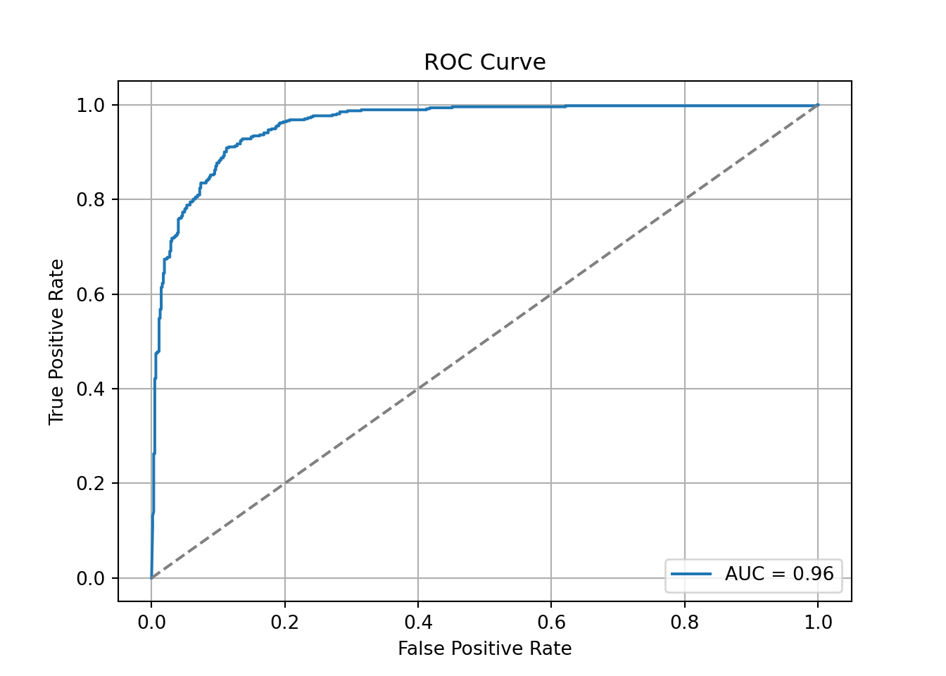
Similar to the sections on model assessment for categorical data, we can use the area under the ROC curve to help evaluate the predictions from the model. We can use the predict_proba function to calculate the predicted probabilities for our data. We only want the probability of a 1 so we will grab the second column (indexed 1 in Python) from the predictions.
From there we can then use the roc_curve and roc_auc_score functions to calculate the ROC curve as well as the area under the ROC curve.
Although rather high with an AUC of 0.96, this Naïve Bayes model did not perform as well as the logistic regression model we evaluated earlier. However, it was rather close and much quicker and easier to build so there are some advantages to it.
If we wanted to tune the Naïve Bayes model parameters, we will need to use the train function from the caret package. The train function will only apply the Naïve Bayes classifier to a categorical target variable. Other functions in R can apply it to a continuous target, but that is not really recommended.
We will create a categorical target variable called bonus that imagines homes selling for more than $175,000 nets the real estate agent a bonus. If bonus takes a value of 1, the house sold for more than $175,000 and 0 otherwise.
In the train function we will tune 3 parameters in the expand.grid. We will allow the algorithm to use either a normal distribution or a kernel distribution with the usekernel option. The other tuning parameters a the Laplace correction (fL) and bandwidth adjustment (adjust).
From the output above, the best Naïve Bayes algorithm has a Laplace correction value of 0, a bandwidth adjustment of 0.5, and uses the kernel distributions for continuous predictor variables.
Code
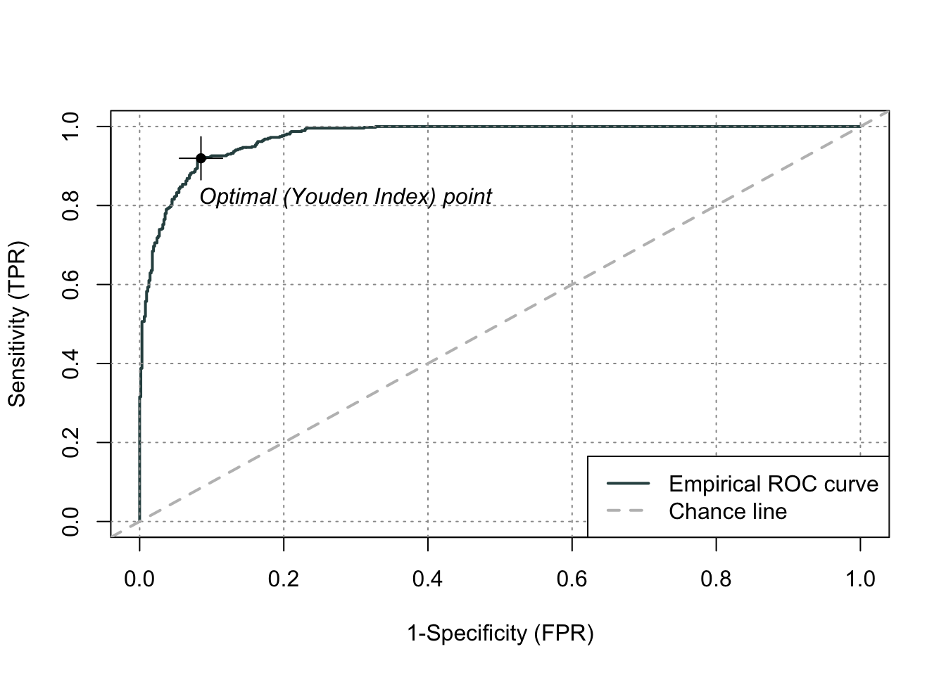
library(ROCit)df_reduced_bonus$p_hat <-predict(nb_ames, type ="prob")[,2]logit_roc <-rocit(df_reduced_bonus$p_hat, df_reduced_bonus$bonus)plot(logit_roc)
Code
summary(logit_roc)
 Method used: empirical
 Number of positive(s): 472
 Number of negative(s): 623
 Area under curve: 0.9723
Although rather high with an AUC of 0.972, this Naïve Bayes model did not perform as well as the logistic regression model we evaluated earlier. However, it was rather close and much quicker and easier to build so there are some advantages to it.
Summary
In summary, Naïve Bayes models are good models to use for prediction, but explanation becomes more difficult and complex. Some of the advantages of using Naïve Bayes:
Very simple to implement
Good at predictions (especially good classification for few categories)
Performs best with categorical variables / text
Fast computational time
Robust to noise and irrelevant variables
There are some disadvantages though:
Independence assumption
Careful about normality assumption for continuous variables
Requires more memory storage than most models
Trust predicted categories more than probabilities
Source Code
---title: "Naive Bayes Model"format: html: code-fold: show code-tools: trueeditor: visual---```{r}#| include: false#| warning: false#| error: false#| message: falselibrary(reticulate)reticulate::use_condaenv("wfu_fall_ml", required =TRUE)``````{python}#| include: false#| warning: false#| error: false#| message: falsefrom sklearn.datasets import fetch_openmlimport pandas as pdfrom sklearn.feature_selection import SelectKBest, f_classifimport numpy as npimport matplotlib.pyplot as plt# Load Ames Housing datadata = fetch_openml(name="house_prices", as_frame=True)ames = data.frame# Remove Business Logic Variablesames = ames.drop(['Id', 'MSSubClass','Functional','MSZoning','Neighborhood', 'LandSlope','Condition2','OverallCond','RoofStyle','RoofMatl','Exterior1st','Exterior2nd','MasVnrType','MasVnrArea','ExterCond','BsmtCond','BsmtExposure','BsmtFinType1','BsmtFinSF1','BsmtFinType2','BsmtFinSF2','BsmtUnfSF','Electrical','LowQualFinSF','BsmtFullBath','BsmtHalfBath','KitchenAbvGr','GarageFinish','SaleType','SaleCondition'], axis=1)# Remove Missingness Variablesames = ames.drop(['PoolQC', 'MiscFeature','Alley', 'Fence'], axis=1)# Impute Missingness for Categorical Variablescat_cols = ames.select_dtypes(include=['object', 'category']).columnsames[cat_cols] = ames[cat_cols].fillna('Missing')# Remove Low Variability Variablesames = ames.drop(['Street', 'Utilities','Heating'], axis=1)# Train / Test Splitfrom sklearn.model_selection import train_test_splittrain, test = train_test_split(ames, test_size =0.25, random_state =1234)# Impute Missing for Continuous Variablesnum_cols = train.select_dtypes(include='number').columnsfor col in num_cols:if train[col].isnull().any():# Create missing flag column train[f'{col}_was_missing'] = train[col].isnull().astype(int)# Impute with median median = train[col].median() train[col] = train[col].fillna(median)# Prepare X and y Objectsimport statsmodels.api as smpredictors = train.drop(columns=['SalePrice'])predictors = pd.get_dummies(predictors, drop_first=True)predictors = predictors.astype(float)predictors = predictors.drop(['GarageType_Missing', 'GarageQual_Missing','GarageCond_Missing'], axis=1)X = predictorsy = train['SalePrice']y_log = np.log(train['SalePrice'])# Initial Variable Selectionselector = SelectKBest(score_func=f_classif, k='all') selector.fit(X, y)pval_df = pd.DataFrame({'Feature': X.columns,'F_score': selector.scores_,'p_value': selector.pvalues_})selected_features = pval_df[pval_df['p_value'] <0.009]['Feature']X_reduced = X[selected_features.tolist()]``````{r}#| include: false#| warning: false#| error: false#| message: falsetrain = py$traintest = py$testX_reduced = py$X_reducedy = py$yy_log = py$y_lognames(X_reduced)[names(X_reduced) =="1stFlrSF"] <-"FirstFlrSF"names(X_reduced)[names(X_reduced) =="2ndFlrSF"] <-"SecondFlrSF"names(X_reduced)[names(X_reduced) =="3SsnPorch"] <-"ThreeStoryPorch"```# General IdeaNaïve Bayes classification is a popular algorithm for predicting a categorical target variable. When using algorithms to classify observations there are two different sources of information that we can use:1. Similarity to other observations based on certain metrics/variables2. Past decisions on classifications of observations like itThe first source of information is the common, frequentist approach to modeling. It predicts values of the target variable in each observation based on predictor variable values. Observations with similar predictor variable values will have similar target variable predictions. The second source of information incorporates a Bayesian approach to modeling in addition to the first source of information. This second source of information uses the information that we know about the population as a whole and previous classifications of observations.This is probably best seen through an example. Imagine we had the scatterplot of data below. In this scatterplot, we have two classes of observations we are trying to predict - green and blue.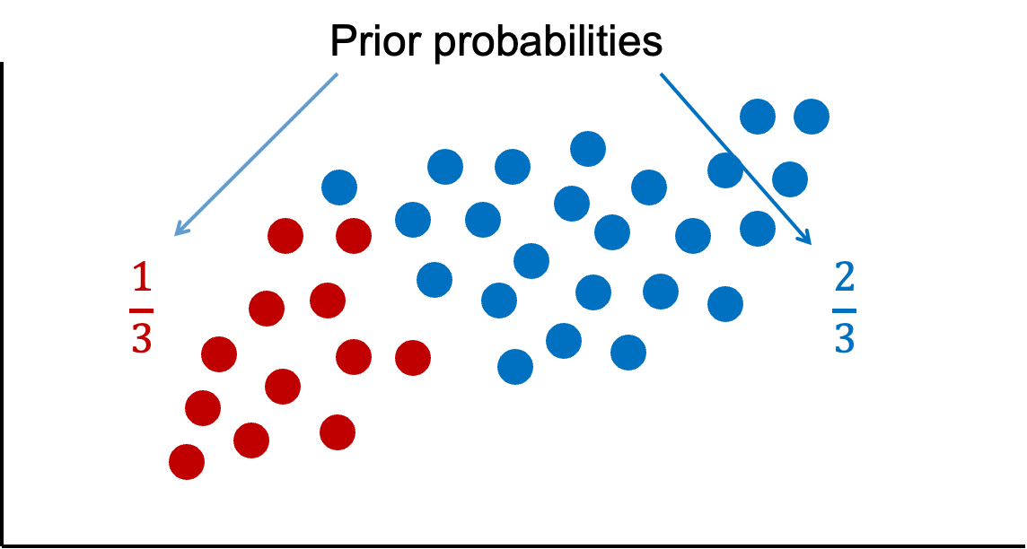{fig-align="center" width="7in"}Let's look at that second source of information - previous information about the classification. Overall in our data set, there are twice as many blues as there are greens. These probabilities are called **prior probabilities**.Now imagine we had a new observation that we wanted to classify.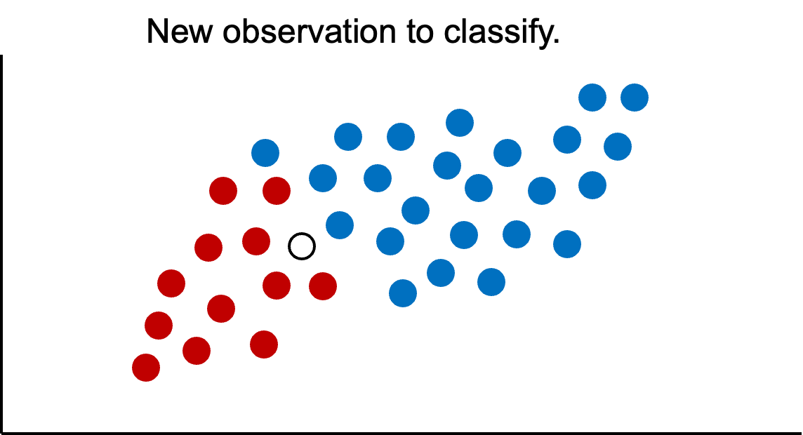{fig-align="center" width="7in"}If we were to use only our previous information about the data, we would guess this new point is blue because historically we have had more blues than greens in the overall population. However, let's bring in the first piece of information - looking at observations with similar characteristics. We can define these observations visually, by looking at observations that are narrowly around the point of interest.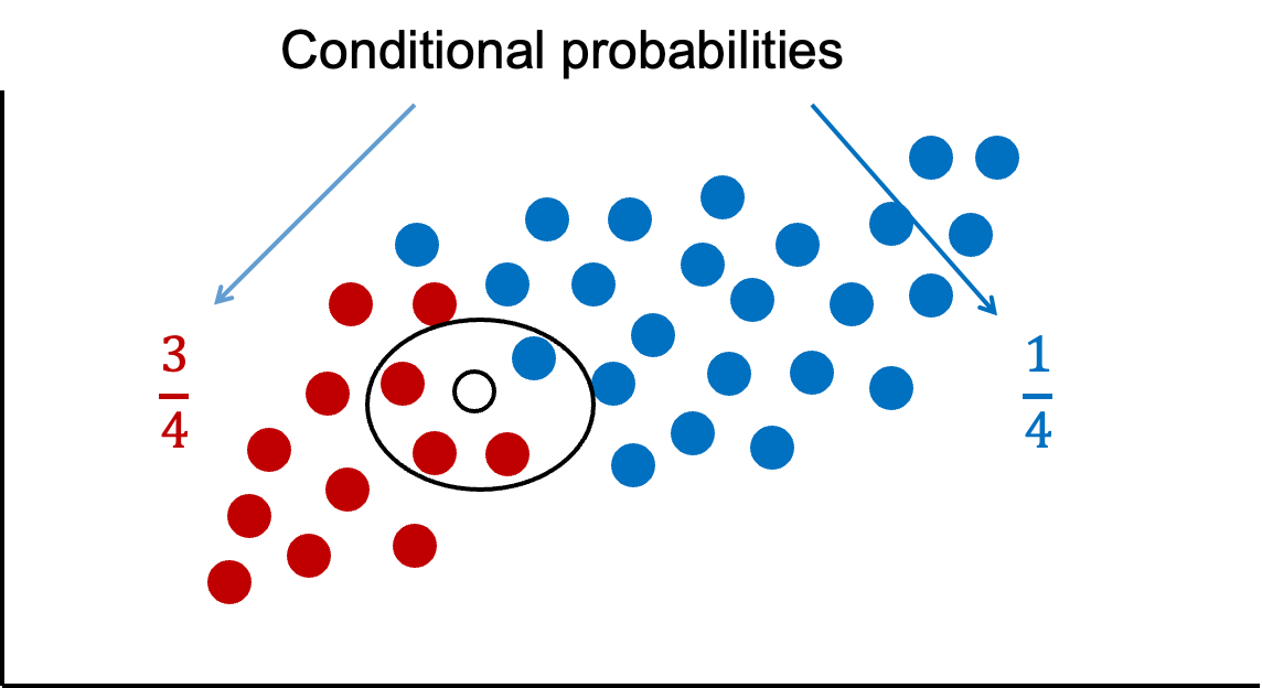{fig-align="center" width="7in"}If we were only to look at observations that are similar as this new observation (the points in the oval), then we would see that there are 3 times more green observations than blue observations. These probabilities are called **conditional probabilities**. If we were to only use this information from similar observations in the data, we would guess this new point is green because there are more greens than blues that look like our new data point.Naïve Bayes combines both of these pieces of information together. We will multiply our prior probabilities by our conditional probabilities.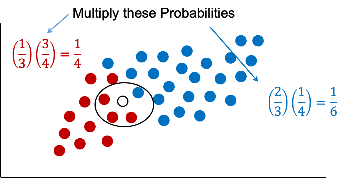{fig-align="center" width="7in"}The downside of this is that these probabilities are not as intuitive since they do not sum up to 1. Therefore, these probabilities are scaled to make their sum equal to 1 and their values more interpretable.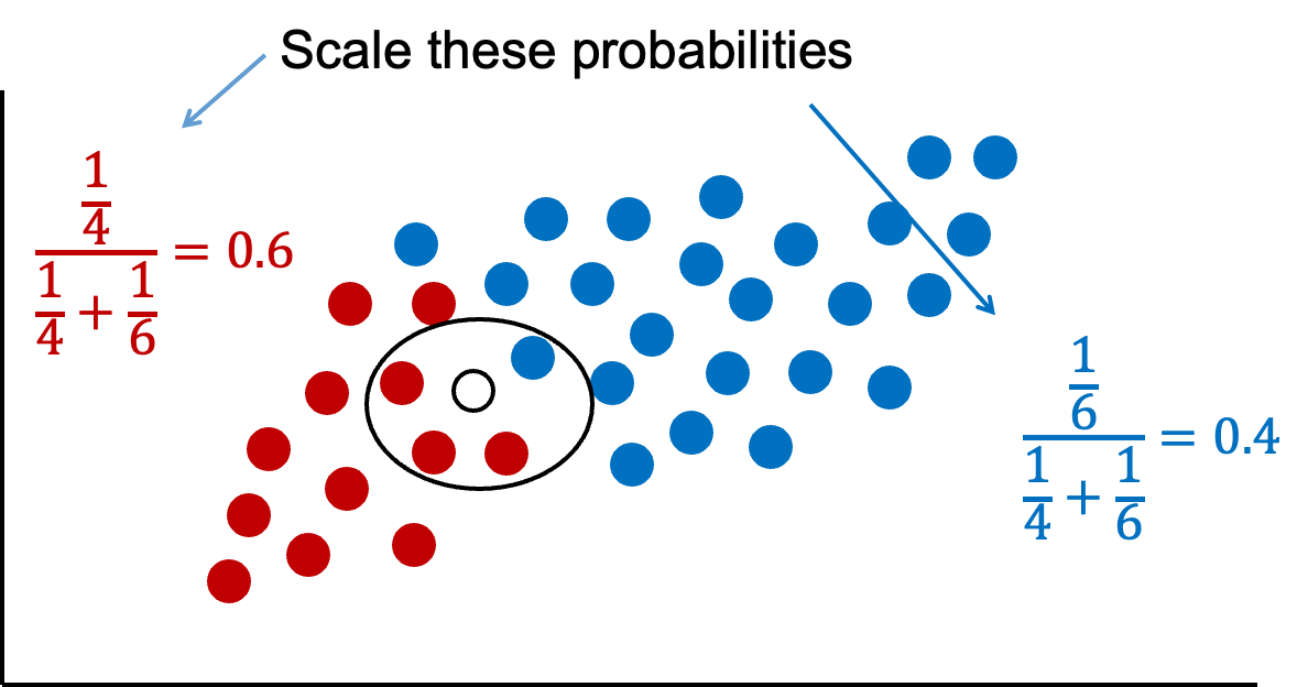{fig-align="center" width="7in"}Now we have final probabilities (called **posterior probabilities**) of both green and blue for our new observation we are trying to classify. Based on the math above, there is a 60% chance the new observation is green and a 40% chance it is blue. If we only use a frequentist approach (the first source of information), we would more strongly think the new observation is green since 75% of the data that looks like that new point is green. However, the Bayesian side of the problem brings in our prior information where 67% of the overall data is blue. Our final guess is still green, but it is not as high as before because of the correction from the prior data - our second source of information.One big assumption of the Naïve Bayes classification method is rather hard to accept - predictor variables are independent in their effects on the classification, or in other words, no interactions. This assumption is the "naïve" part of the algorithm. However, in practice, this assumption doesn't seem to drastically impact our final posterior probability predictions.# Underlying MathBayesian classifiers are based on Bayes' Theorem:$$P(y|x_1, x_2, \ldots, x_p) = \frac{P(y) \times P(x_1, x_2, \ldots, x_p|y)}{P(x_1, x_2, \ldots, x_p)}$$The Naïve Bayes classifier assumes that the effect of the inputs are independent of one another (that "naïve" assumption mentioned above). Remember the rule about probabilities and independent events:$$P(A \cap B) = P(A) \times P(B)$$Based on this rule, Bayes' Theorem now becomes:$$P(y|x_1, x_2, \ldots, x_p) = \frac{P(y) \times P(x_1|y) \times \cdots P(x_p|y)}{P(x_1) \times \cdots P(x_p)}$$This makes the math much easier to calculate!Let's work through a simple example based on the following table:| Size | Color | Accident ||:------:|:-----:|:--------:|| Large | Blue | Yes || Large | Green | Yes || Large | Blue | No || Large | Blue | No || Medium | Green | Yes || Medium | Blue | Yes || Medium | Green | Yes || Small | Blue | No || Small | Green | Yes || Small | Green | No |We will try to predict the probability of getting into an accident based on two variables - size of car and color of car.Imagine we had a new observation that is a blue, medium car. Let's use Bayes' Theorem to calculate the probabilities of a Yes and No for accident:$$P(Y|M \& B) = \frac{P(Y) \times P(M|Y) \times P(B|Y)}{P(M) \times P(B)}$$From the table above we can see that there are 6 out of 10 cars that get into an accident, $P(Y) = 0.6$. Of the cars that get into an accident, 3 of the 6 are medium, $P(M|Y) = 0.5$. Of the cars that get into an accident, 2 of the 6 are blue, $P(B|Y) = 0.333$. Of all of the cars, 3 out of the 10 are medium, $P(M) = 0.3$, and 5 out of 10 are blue, $P(B) = 0.5$. Inputting these values into the equation above, we get a probability of getting into an accident given the car is blue and medium as $P(Y|M \& B) = 0.667$.Let's do the same thing for the probability of not getting into an accident given the car is blue and medium:$$P(N|M \& B) = \frac{P(N) \times P(M|N) \times P(B|N)}{P(M) \times P(B)}$$We can see that 4 out of the 10 cars did **not** get into an accident, $P(N) = 0.4$. Of the cars that did not get into an accident, 0 out of the 4 were medium sized, $P(M|N) = 0$. This poses and problem. With this 0 in the calculation, the probability of not getting into an accident is forced to 0. This is more likely due to our small sample size and not truly representative of the population as a whole. This is similar to the problem of quasi-complete separation in logistic regression. Luckily, the Naïve Bayes algorithm has a built in mechanism to handle this. The algorithm uses a Laplace correction, essentially adding a small constant to each of the counts to prevent any 0 probability calculations.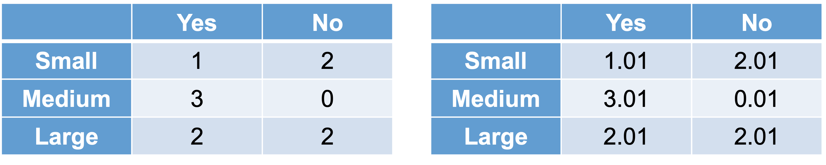{fig-align="center" width="6in"}For example, instead of a classification table comparing size of car to accident (yes or no) as our original data has it (the left table above), the algorithm instead will add a small constant to each cell (the right table above). Now the calculation for the probability of a medium car given no accident becomes $P(M|N) = 0.01/4.03 = 0.0025$. Now we can fill out the rest easily, $P(B|N) = 0.75$, $P(M) = 0.3$, and $P(B) = 0.5$. Inputting these values into the equation above, we get a probability of not getting into an accident given the car is blue and medium as $P(N|M \& B) = 0.005$.Remember, these are not scaled. If we scale these probabilities, our probability of getting into an accident given the car is blue and medium is 0.993. The probability of not getting into an accident is now 0.007.# Fitting Naive BayesWe worked through the Naïve Bayes algorithm when we had a categorical target and categorical predictor variable. In this situation, we determine the predicted probability of each target category based on cross-tabulation tables of each variable with the target variable (same idea as previous section). However, when we have numeric predictor variables, the process is a little different. With a continuous predictor variable, the algorithm determines the probability on values from either a Normal (Gaussian) distribution with the same mean and standard deviation as our data **or** a kernel density estimation of the data.Although the Naïve Bayes classifier was designed for target variables that are categorical, some softwares can also apply the algorithm to continuous target variables as well. In these situations, the software actually treats the continuous target variable as a categorical variable with a large number of categories. The value of the target variable that is the highest probability will be the prediction for the continuous target variable. However, this process is not really recommended as a good strategy for continuous target variables since it would only be able to predict values that were previously seen.Let's see this in each software!::: {.panel-tabset .nav-pills}## PythonIf we wanted to build the Naïve Bayes model in Python, we will need to use the `GaussianNB` function from the `sklearn.naive_bayes` package. The `GaussianNB` function will only apply the Naïve Bayes classifier to a categorical target variable.We will create a categorical target variable called *bonus* that imagines homes selling for more than \$175,000 nets the real estate agent a bonus. If *bonus* takes a value of 1, the house sold for more than \$175,000 and 0 otherwise. This is created in Python below like we did in the section on logistic regression. The `GaussianNB` function uses the Normal distribution for continuous predictor variables. We use the `GaussianNB` and `fit` functions on our training data in the typical Python structure with a data frame of predictor variables and a target vector.```{python}#| warning: false#| error: false#| message: falsefrom sklearn.naive_bayes import GaussianNBy_bonus = (y >175000).astype(int)gnb = GaussianNB()gnb.fit(X_reduced, y_bonus)```Similar to the sections on model assessment for categorical data, we can use the area under the ROC curve to help evaluate the predictions from the model. We can use the `predict_proba` function to calculate the predicted probabilities for our data. We only want the probability of a 1 so we will grab the second column (indexed 1 in Python) from the predictions.From there we can then use the `roc_curve` and `roc_auc_score` functions to calculate the ROC curve as well as the area under the ROC curve.```{python}#| warning: false#| error: false#| message: falsetrain['p_hat'] = gnb.predict_proba(X_reduced)[:, 1]import matplotlib.pyplot as pltfrom sklearn.metrics import roc_curve, roc_auc_score, RocCurveDisplayfpr, tpr, thresholds = roc_curve(y_bonus, train['p_hat'])auc = roc_auc_score(y_bonus, train['p_hat'])plt.plot(fpr, tpr, label=f"AUC = {auc:.2f}")plt.plot([0, 1], [0, 1], linestyle="--", color="gray") # chance lineplt.xlabel("False Positive Rate")plt.ylabel("True Positive Rate")plt.title("ROC Curve")plt.legend()plt.grid(True)plt.show()```Although rather high with an AUC of 0.96, this Naïve Bayes model did not perform as well as the logistic regression model we evaluated earlier. However, it was rather close and much quicker and easier to build so there are some advantages to it.## RIf we wanted to tune the Naïve Bayes model parameters, we will need to use the `train` function from the `caret` package. The `train` function will only apply the Naïve Bayes classifier to a categorical target variable. Other functions in R can apply it to a continuous target, but that is not really recommended.We will create a categorical target variable called *bonus* that imagines homes selling for more than \$175,000 nets the real estate agent a bonus. If *bonus* takes a value of 1, the house sold for more than \$175,000 and 0 otherwise.```{r}#| warning: false#| error: false#| message: falsey_bonus <-ifelse(y >175000, 1, 0)df_reduced_bonus <-data.frame(bonus = y_bonus, X_reduced)```In the `train` function we will tune 3 parameters in the `expand.grid`. We will allow the algorithm to use either a normal distribution or a kernel distribution with the `usekernel` option. The other tuning parameters a the Laplace correction (`fL`) and bandwidth adjustment (`adjust`).```{r}#| warning: false#| error: false#| message: falselibrary(caret)library(klaR)tune_grid <-expand.grid(usekernel =c(TRUE, FALSE),fL =c(0, 0.5, 1),adjust =c(0.1, 0.5, 1))set.seed(12345)nb_ames <- caret::train(factor(bonus) ~ ., data = df_reduced_bonus,method ="nb", tuneGrid = tune_grid,trControl =trainControl(method ='cv', number =10))nb_ames$bestTune```From the output above, the best Naïve Bayes algorithm has a Laplace correction value of 0, a bandwidth adjustment of 0.5, and uses the kernel distributions for continuous predictor variables.```{r}#| warning: false#| error: false#| message: falselibrary(ROCit)df_reduced_bonus$p_hat <-predict(nb_ames, type ="prob")[,2]logit_roc <-rocit(df_reduced_bonus$p_hat, df_reduced_bonus$bonus)plot(logit_roc)summary(logit_roc)```Although rather high with an AUC of 0.972, this Naïve Bayes model did not perform as well as the logistic regression model we evaluated earlier. However, it was rather close and much quicker and easier to build so there are some advantages to it.:::# SummaryIn summary, Naïve Bayes models are good models to use for prediction, but explanation becomes more difficult and complex. Some of the advantages of using Naïve Bayes:- Very simple to implement- Good at predictions (especially good classification for few categories)- Performs best with categorical variables / text- Fast computational time- Robust to noise and irrelevant variablesThere are some disadvantages though:- Independence assumption- Careful about normality assumption for continuous variables- Requires more memory storage than most models- Trust predicted categories more than probabilities