A newer algorithm has come onto the scene that tries to have the predictive power seen in XGBoost models but maintain the kind of interpretability that GAM models have. This model is called the explainable boosting machine (EBM).
We covered GAM’s in a previous section, but as a reminder, GAM’s provide a general framework for the adding of non-linear functions together instead of the typical linear structure. The structure of GAM’s are the following:
The \(f_i(x_i)\) functions are complex, nonlinear functions on the predictor variables. GAM’s add these complex, yet individual functions together. This allows for many complex relationships to try and model with to potentially predict your target variable better.
EBM’s use machine learning algorithms (like random forests and boosting trees) to build these individual pieces, \(f_i (x_i)\), before adding them together in the GAM. To do this, they build out the same GBM structure but only use one variable at a time. The idea behind the GBM is to build a simple model to predict the target (much like a decision tree or even decision stump):
\[
y = g_1(x_1) + \varepsilon_1
\]
However, in the EBM that simple model is built only off of one variable, say \(x_1\). That simple model has an error of \(\varepsilon_1\). The next step is to try to predict that error with another simple model only using one other variable, say \(x_2\):
\[
\varepsilon_1 = g_2(x_2) + \varepsilon_2
\]
This model has an error of \(\varepsilon_2\). We can continue to add model after model, each one predicting the error (residuals) from the previous round, but only ever using one variable:
We will continue this process until we use all of the variables. We will then repeat this process in a round robin format, but still looking at the residuals from the previous set of models:
This will be repeated in a round robin format for thousands of iterations similar to a random forest approach where size of the iterations help find all the signal. We will apply a small learning rate to each of the subsequent models (each trees contribution to the running residual is scaled by a small number) so that the order of the variables will not matter. For each of the small models containing only the variable \(x_1\), \(g_1(x_1)\), \(g_{1^*}(x_1)\), \(g_{1^{**}}(x_1)\), etc. , we will aggregate them together to form our idea of the overall relationship between \(x_1\) and \(y\), our \(f_1(x_1)\) for our GAM:
We will then repeat this process for all of the variables in the model. Essentially, we are developing each of the pieces of the GAM (the individual variable relationships) and then adding them together to form our overall model.
These allow for individually developed relationships for variables which makes the interpretability more similar to that of the traditional GAM’s, but with the predictive power of the more advanced machine learning boosting algorithms.
Python has a much more developed version of the EBM model than R does. It can build an EBM with either a continuous or categorical target variable. Let’s see examples of both.
First, we will try to predict our housing prices in Ames, Iowa as before. To do this we will use the interpret and interpret.glassbox packages and the ExplainableBoostingRegressor function. In the ExplainableBoostingRegressor function we limit the number of interactions we want to allow in the model. By default, this function will allow up to 90% of the count of variables as the number of possible interactions. Similar to other Python functions we have used, we need the training predictor variables in one object and the target variable in another. These will be passed to the .fit portion of the code below.
In a Jupyter environment, please rerun this cell to show the HTML representation or trust the notebook. On GitHub, the HTML representation is unable to render, please try loading this page with nbviewer.org.
Parameters
feature_names
None
feature_types
None
max_bins
1024
max_interaction_bins
64
interactions
3
exclude
None
validation_size
0.15
outer_bags
14
inner_bags
0
learning_rate
0.04
greedy_ratio
10.0
cyclic_progress
False
smoothing_rounds
500
interaction_smoothing_rounds
100
max_rounds
50000
early_stopping_rounds
100
early_stopping_tolerance
1e-05
callback
None
min_samples_leaf
4
min_hessian
0.0
reg_alpha
0.0
reg_lambda
0.0
max_delta_step
0.0
gain_scale
5.0
min_cat_samples
10
cat_smooth
10.0
missing
'separate'
max_leaves
2
monotone_constraints
None
objective
'rmse'
n_jobs
1
random_state
42
To build a model with a categorical target we can create a categorical target variable called bonus that imagines homes selling for more than $175,000 nets the real estate agent a bonus. If bonus takes a value of 1, the house sold for more than $175,000 and 0 otherwise. This was created below.
Code
y_bonus = (y >175000).astype(int)
Since we have a categorical target variable instead, we will use the ExplainableBoostingClassifier function. In the ExplainableBoostingClassifier function we limit the number of interactions we want to allow in the model. By default, this function will allow up to 90% of the count of variables as the number of possible interactions. Similar to other Python functions we have used, we need the training predictor variables in one object and the target variable in another. These will be passed to the .fit portion of the code below.
Code
from interpret.glassbox import ExplainableBoostingClassifierebm_ames_c = ExplainableBoostingClassifier(interactions =3, n_jobs =1)ebm_ames_c.fit(X_reduced, y_bonus)
In a Jupyter environment, please rerun this cell to show the HTML representation or trust the notebook. On GitHub, the HTML representation is unable to render, please try loading this page with nbviewer.org.
Parameters
feature_names
None
feature_types
None
max_bins
1024
max_interaction_bins
64
interactions
3
exclude
None
validation_size
0.15
outer_bags
14
inner_bags
0
learning_rate
0.015
greedy_ratio
10.0
cyclic_progress
False
smoothing_rounds
75
interaction_smoothing_rounds
75
max_rounds
50000
early_stopping_rounds
100
early_stopping_tolerance
1e-05
callback
None
min_samples_leaf
4
min_hessian
0.0001
reg_alpha
0.0
reg_lambda
0.0
max_delta_step
0.0
gain_scale
5.0
min_cat_samples
10
cat_smooth
10.0
missing
'separate'
max_leaves
2
monotone_constraints
None
objective
'log_loss'
n_jobs
1
random_state
42
R has an implementation of the EBM model with the interpret package. However, that package will only apply the EBM model to a binary target variable. The new ebm package wraps the most recent Python InterpretML engine and can actually predict both continuous and categorical target variables.
First, we will try to predict our housing prices in Ames, Iowa as before. To do this we will use the ebm package and the ebm function. In the ebm function we limit the number of interactions we want to allow in the model. By default, this function will allow up to 90% of the count of variables as the number of possible interactions. Similar to other R functions we have used, we need the training predictor variables and the target variable in one data frame. This will be passed to the data option in the code below. Lastly, we will specify the objective = "rmse" option to signal to the ebm function that we have a continuous target variable.
To build a model with a categorical target we can create a categorical target variable called bonus that imagines homes selling for more than $175,000 nets the real estate agent a bonus. If bonus takes a value of 1, the house sold for more than $175,000 and 0 otherwise. This was created below.
Code
y_bonus <-ifelse(y >175000, 1, 0)
Even if we have a categorical target variable instead, we will still use the ebm function. In the ebm function we limit the number of interactions we want to allow in the model. By default, this function will allow up to 90% of the count of variables as the number of possible interactions. Similar to other R functions we have used, we need the training predictor variables and the target variable in one data frame. This will be passed to the data option in the code below. Lastly, we will specify the objective = "log_loss" option to signal to the ebm function that we have a binary target variable.
Now we have an EBM model built. We can use some of the functionality of that model to try and interpret the variables. Remember the GAM structure to the EBM as described above? This allows for individually developed relationships for variables which makes the interpretability more similar to that of the traditional GAM’s, but with the predictive power of the more advanced machine learning boosting algorithms.
Python has a robust set of interpretations for the EBM model. From the interpret package we will need the show, InlineProvider, and set_visualize_provider functions. First, we use the set_visualize_provider function with the InlineProvider function to scan our environment and use the best visualization setup for our environment. From there we can start to visualize the model features.
First, we will use the explain_global() function on the EBM model object created above. This will calculate all of the global interpretations from our model. From there we can use the visualize() function as well as the show function to plot the global importance.
From the plot above we have a global importance score for each variable. Let’s look at the 4th variable, GrLivaArea. This variable has a weighted Mean Absolute Score of 7,080.72. This has some interpretive value! This means that, on average, the GrLivaArea variable moved predictions in some direction by $7,080.72. This average movement was the 4th largest of any variable in terms of impact. We can see the same thing for the remaining variables.
If we wanted to explore the variables on an individual level we can call a specific variable by number in the visualize function as shown below. The variables are listed in the order they are put into the model, however, the continuous variables are all grouped first, followed by the categorical variables. For example, the GrLivArea variable is the 9th (index value of 8) continuous predictor variable put in our model.
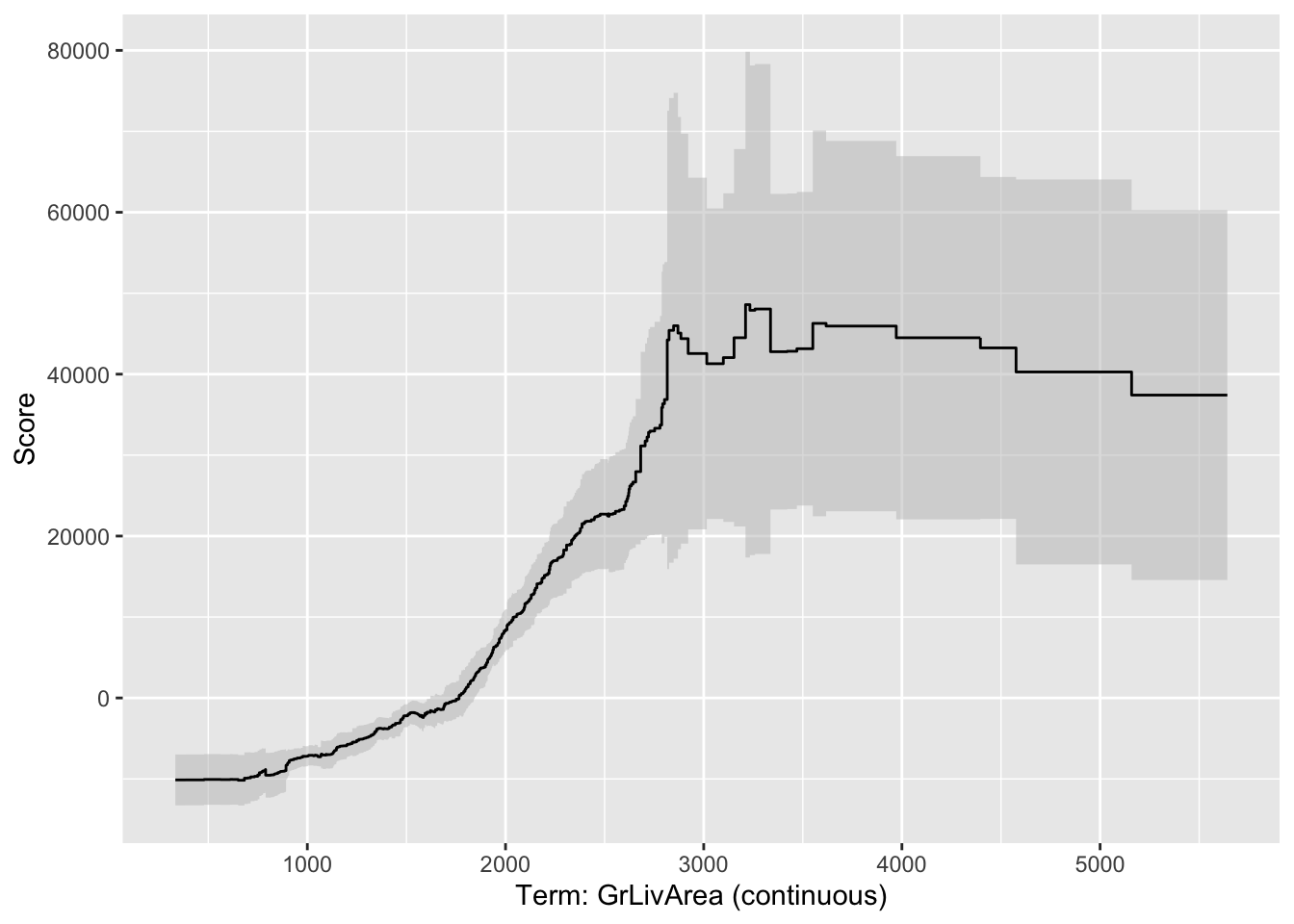
From the plot above we can see the predicted relationship between the variable GrLivArea and SalePrice. This nonlinear and complex relationship is similar to the plot we saw earlier with the GAMs, random forests, and XGBoost models. This shouldn’t be too surprising. All of these algorithms are trying to relate these two variables together, just in different ways. The density plot below this graph is just a histogram of the values of GrLivArea.
For completeness sake, below is the same code, but for the EBM model built on our binary target variable of bonus. First, we will use the explain_global() function on the EBM model object created above. This will calculate all of the global interpretations from our model. From there we can use the visualize() function as well as the show function to plot the global importance.
From the plot above we have a global importance score for each variable. Let’s look at the first variable, GrLivArea. This variable has a weighted Mean Absolute Score of 0.693. Unlike with the continuous target variable, this doesn’t have as nice of an interpretation. This means that, on average, the GrLivArea variable moved the natural log of the odds (logit) in some direction by 0.693. This average movement was larger than any other variable in terms of impact. We can see the same thing for the remaining variables.
If we wanted to explore the variables on an individual level we can call a specific variable by number in the visualize function as shown below. The variables are listed in the order they are put into the model, however, the continuous variables are all grouped first, followed by the categorical variables. For example, the GrLivArea variable is the 9th (index value of 8) continuous predictor variable put in our model.
Since Python has a robust set of interpretations for the EBM model, R’s ebm function imports those for use in R.
First, we will use the plot() function on the EBM model object created above. This will calculate all of the global interpretations from our model and plot the global importance.
Code
plot(ebm_ames)
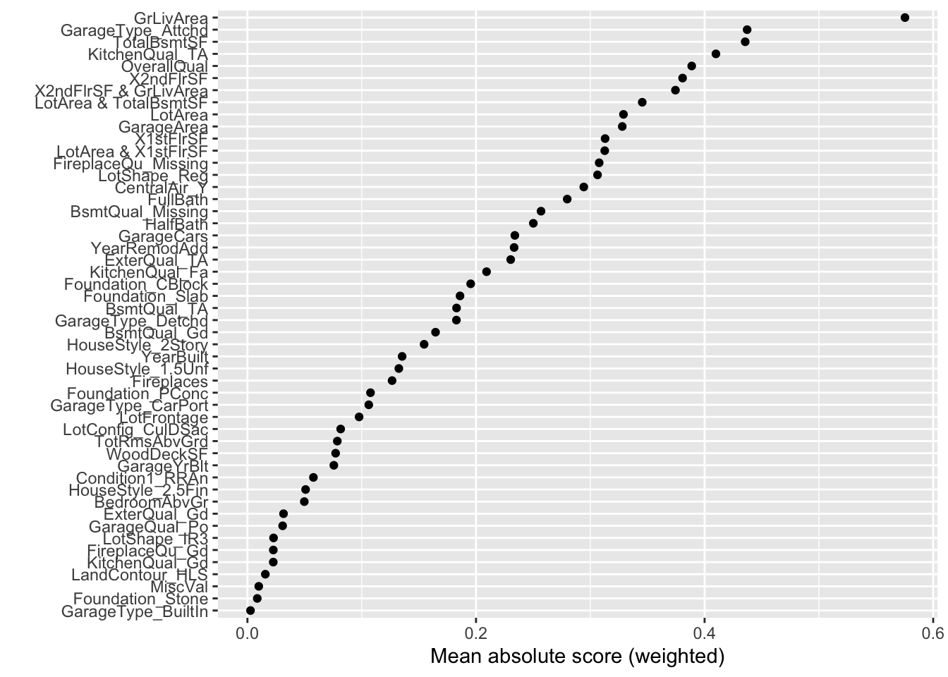
From the plot above we have a global importance score for each variable. Let’s look at the 4th variable, GrLivaArea. We need to extract these numeric values to see what they actually are.
This variable has a weighted Mean Absolute Score of 7,020.24. This has some interpretive value! This means that, on average, the GrLivaArea variable moved predictions in some direction by $7,020.24. This average movement was the 4th largest of any variable in terms of impact. We can see the same thing for the remaining variables.
If we wanted to explore the variables on an individual level we can call a specific variable by name in the plot function as shown below. Here we will use the GrLivArea variable.
Code
plot(ebm_ames, "GrLivArea")
This nonlinear and complex relationship between GrLivArea and SalePrice is similar to the plot we saw earlier with the GAMs, random forests, and XGBoost models. This shouldn’t be too surprising. All of these algorithms are trying to relate these two variables together, just in different ways.
For completeness sake, below is the same code, but for the EBM model built on our binary target variable of bonus. First, we will use the plot() function on the EBM model object created above. This will calculate all of the global interpretations from our model and plot the global importance as well as print out all of their values.
From the plot above we have a global importance score for each variable. Let’s look at the first variable, GrLivArea. This variable has a weighted Mean Absolute Score of 0.575. Unlike with the continuous target variable, this doesn’t have as nice of an interpretation. This means that, on average, the GrLivArea variable moved the natural log of the odds (logit) in some direction by 0.575. This average movement was larger than any other variable in terms of impact. We can see the same thing for the remaining variables.
If we wanted to explore the variables on an individual level we can call a specific variable by name in the plot function as shown below. Here we will use the GrLivArea variable.
Code
plot(ebm_ames_c, "GrLivArea")
Variable Selection
Another thing to tune would be which variables to include in the EBM model. By default, EBM models use all the variables since they are aggregated across all the trees used to build the model. There are a couple of ways to perform variable selection for EBM’s:
Many permutations of including/excluding variables
Compare variables to random variable
The first approach is rather straight forward but time consuming because you have to try and build models over and over again taking a variable out each time. The second approach is much easier to try. In that second approach we will create a completely random variable and put it in the model. We will then look at the variable importance of all the variables. The variables that are below the random variable should be considered for removal.
To create a random variable in Python we will first create a new data.frame called X_train_r. We will then add a variable called random with the random.normal function from numpy. We then build an EBM model in the same way we did previously and check the variable importance.
Code
import numpy as npX_reduced_r = X_reduced.copy()X_reduced_r['random'] = np.random.normal(0, 1, X_reduced.shape[0])
Instead of plotting the variable importance for the variables we will just print out a list of the importance for each variable using the term_importance and term_name functions.
In a Jupyter environment, please rerun this cell to show the HTML representation or trust the notebook. On GitHub, the HTML representation is unable to render, please try loading this page with nbviewer.org.
Term LotFrontage importance: 1911.2196001889995
Term LotArea importance: 4078.3705995983287
Term OverallQual importance: 8674.311808154987
Term YearBuilt importance: 3271.844787495058
Term YearRemodAdd importance: 5092.431638877743
Term TotalBsmtSF importance: 8230.018744843283
Term 1stFlrSF importance: 5098.7904553846
Term 2ndFlrSF importance: 4898.432395187888
Term GrLivArea importance: 6812.287298823504
Term FullBath importance: 1205.0933408637966
Term HalfBath importance: 3436.5111924538187
Term BedroomAbvGr importance: 1982.6697005053638
Term TotRmsAbvGrd importance: 1392.281019034489
Term Fireplaces importance: 2976.758352025514
Term GarageYrBlt importance: 889.2763820628845
Term GarageCars importance: 3622.98550314814
Term GarageArea importance: 3988.667537833611
Term WoodDeckSF importance: 2389.857398877394
Term MiscVal importance: 104.47556023104697
Term LotShape_IR3 importance: 364.0772070197787
Term LotShape_Reg importance: 1852.0992367748465
Term LandContour_HLS importance: 441.48646930995835
Term LotConfig_CulDSac importance: 1156.8798679966085
Term Condition1_RRAn importance: 39.354632844855864
Term HouseStyle_1.5Unf importance: 29.320870115304
Term HouseStyle_2.5Fin importance: 31.908299772281115
Term HouseStyle_2Story importance: 1910.1327065254552
Term ExterQual_Gd importance: 295.8073540639061
Term ExterQual_TA importance: 4663.713196138708
Term Foundation_CBlock importance: 98.92478749984117
Term Foundation_PConc importance: 3589.866793732971
Term Foundation_Slab importance: 93.23440656599533
Term Foundation_Stone importance: 29.027908775950575
Term BsmtQual_Gd importance: 4854.619189142825
Term BsmtQual_Missing importance: 775.8109974815611
Term BsmtQual_TA importance: 7012.348061124197
Term CentralAir_Y importance: 1101.6461639979964
Term KitchenQual_Fa importance: 1357.9663838627246
Term KitchenQual_Gd importance: 6850.010518354791
Term KitchenQual_TA importance: 10797.50927947989
Term FireplaceQu_Gd importance: 667.0323349218435
Term FireplaceQu_Missing importance: 3068.750683240653
Term GarageType_Attchd importance: 3012.008155838368
Term GarageType_BuiltIn importance: 207.47850443940806
Term GarageType_CarPort importance: 311.9826895117438
Term GarageType_Detchd importance: 228.24337735916174
Term GarageQual_Po importance: 73.34110517404987
Term random importance: 635.1897138729768
Term OverallQual & YearRemodAdd importance: 1380.5748639088504
Term OverallQual & BedroomAbvGr importance: 1126.0783869506001
Term OverallQual & GarageArea importance: 1848.1014638779827
Based on the list above there are 3 variables that fall below the variable importance of the random variable that could be considered for removal from the model.
To create a random variable in R we will just use the rnorm function with a mean of 0, standard deviation of 1 (both defaults) and a count of the number of observations in our training data.
Code
library(dplyr)set.seed(1234)# Copy X_reduced and add a random featureX_reduced_r <- X_reducedX_reduced_r$random <-rnorm(nrow(X_reduced_r), mean =0, sd =1)
We then build the EBM model in the same way we did previously and check the variable importance.
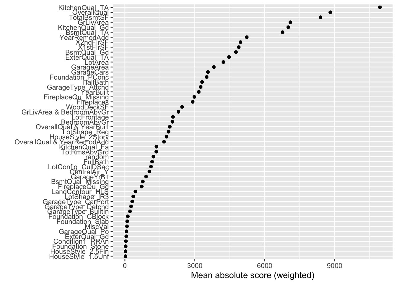
Based on the plot above there are 20 variables that fall below the variable importance of the random variable that could be considered for removal from the model.
Local Interpretability
Another valuable piece of output from the Python functionality of EBM models is the ability to perform local interpretability as well as the global interpretability we saw earlier. Python’s functionality automatically plots these importances while R can only give the raw importance values. Here we will just go over the Python functionality.
The above plot breaks down the individual prediction from the model into how each variable impacts prediction. The plot above breaks down the model’s predictions for that one specific observation into all of the components that contribute to that prediction. For example, the overall quality of the home being a 9 out of 10 contributes $40,701.35 to the predicted price of $315,000.
More details on these kinds of calculations are listed in the Model Agnostic Interpretability section of the notes.
Predictions
Models are nothing but potentially complicated formulas or rules. Once we determine the optimal model, we can score any new observations we want with the equation.
Scoring data does not mean that we are re-running the model/algorithm on this new data. It just means that we are asking the model for predictions on this new data - plugging the new data into the equation and recording the output. This means that our data must be in the same format as the data put into the model. Therefore, if you created any new variables, made any variable transformations, or imputed missing values, the same process must be taken with the new data you are about to score.
For this problem we will score our test dataset that we have previously set aside as we were building our model. The test dataset is for comparing final models and reporting final model metrics. Make sure that you do NOT go back and rebuild your model after you score the test dataset. This would no longer make the test dataset an honest assessment of how good your model is actually doing. That also means that we should NOT just build hundreds of iterations of our same model to compare to the test dataset. That would essentially be doing the same thing as going back and rebuilding the model as you would be letting the test dataset decide on your final model.
Without going into all of the same detail as before, the following code transforms the test dataset we originally created in the same way that we did for the training dataset by dropping necessary variables, making missing value imputations, and getting our same data objects.
Code
predictors_test = test.drop(columns=['SalePrice'])ames_dummied = pd.get_dummies(ames, drop_first=True)test_ids = test.indextest_dummied = ames_dummied.loc[test_ids]predictors_test = test_dummied.astype(float)predictors_test = predictors_test.drop(['GarageType_Missing', 'GarageQual_Missing','GarageCond_Missing'], axis=1)# Impute Missing for Continuous Variablesnum_cols = predictors_test.select_dtypes(include='number').columnsfor col in num_cols:if predictors_test[col].isnull().any(): predictors_test[f'{col}_was_missing'] = predictors_test[col].isnull().astype(int)# Impute with median median = predictors_test[col].median() predictors_test[col] = predictors_test[col].fillna(median)X_test = predictors_testy_test = test['SalePrice']y_test_log = np.log(test['SalePrice'])# Subset the DataFrame to selected featuresX_test_selected = X_test[selected_features].copy()
Now that our data is ready for scoring, we can use the predict function on our model object we created with our EBM model. The only input to the predict function is the dataset we prepared for scoring.
From the sklearn.metrics package we have a variety of model metric functions. We will use the mean_absolute_error (MAE) and mean_absolute_percentage_error (MAPE) metrics like the ones we described in the section on Model Building.
From the above output we can see that the newly created EBM model is not as predictive as the random forest and XGboost models, but more comparable to the linear regression and GAM models.
Model
MAE
MAPE
Linear Regression
$18,160.24
11.36%
Ridge Regression
$19.572.19
12.25%
GAM
$18,154.31
11.40%
Decision Tree
$25,422.52
16.01%
Random Forest
$16,974.22
10.90%
XGBoost
$17,825.07
10.94%
EBM
$18,774.71
11.60%
To make sure that we are using the same test dataset between Python and R we will import our Python dataset here into R. There are a few variables that need to be renamed with the names function to work best in R.
Now that our data is ready for scoring based on the code for the decision tree model, we can use the predict function on our model object we created with our EBM. The only input to the predict function is the dataset we prepared for scoring, but that dataset must be converted into a matrix like we did for building the EBM model.
From the Metrics package we have a variety of model metric functions. We will use the mae (mean absolute error) and mape (mean absolute percentage error) metrics like the ones we described in the section on Model Building.
From the above output we can see that the newly created EBM model is slightly worse than the linear regression and XGBoost models, but comes in behind the random forest model.
Model
MAE
MAPE
Linear Regression
$18,160.24
11.36%
Ridge Regression
$22,040.76
13.37%
GAM
$19,479.79
12.23%
Decision Tree
$22,934.49
13.92%
Random Forest
$16,864.85
10.77%
XGBoost
$18,285.01
11.37%
EBM
$18,801.94
11.64%
Summary
In summary, EBM models are good models to use for prediction and keeps similar interpretability of GAM models. Some of the advantages of using EBM models:
Early results show they are powerful at predicting (almost to the level of XGBoost).
Interpretation available due to GAM nature (individually estimated relationships)
There are some disadvantages though:
Computationally slower than random forests due to sequentially building trees
More tuning parameters than random forests
Limited implementations across all softwares
Source Code
---title: "Explainable Boosting Machine"format: html: code-fold: show code-tools: true self-contained: false embed-resources: falsejupyter: python3engine: knitreditor: visual---```{r}#| include: false#| warning: false#| error: false#| message: falselibrary(reticulate)reticulate::use_condaenv("wfu_fall_ml_ebm_old", required =TRUE)``````{python}#| include: false#| warning: false#| error: false#| message: falsefrom sklearn.datasets import fetch_openmlimport pandas as pdfrom sklearn.feature_selection import SelectKBest, f_classifimport numpy as npimport matplotlib.pyplot as plt# Load Ames Housing datadata = fetch_openml(name="house_prices", as_frame=True)ames = data.frame# Remove Business Logic Variablesames = ames.drop(['Id', 'MSSubClass','Functional','MSZoning','Neighborhood', 'LandSlope','Condition2','OverallCond','RoofStyle','RoofMatl','Exterior1st','Exterior2nd','MasVnrType','MasVnrArea','ExterCond','BsmtCond','BsmtExposure','BsmtFinType1','BsmtFinSF1','BsmtFinType2','BsmtFinSF2','BsmtUnfSF','Electrical','LowQualFinSF','BsmtFullBath','BsmtHalfBath','KitchenAbvGr','GarageFinish','SaleType','SaleCondition'], axis=1)# Remove Missingness Variablesames = ames.drop(['PoolQC', 'MiscFeature','Alley', 'Fence'], axis=1)# Impute Missingness for Categorical Variablescat_cols = ames.select_dtypes(include=['object', 'category']).columnsames[cat_cols] = ames[cat_cols].fillna('Missing')# Remove Low Variability Variablesames = ames.drop(['Street', 'Utilities','Heating'], axis=1)# Train / Test Splitfrom sklearn.model_selection import train_test_splittrain, test = train_test_split(ames, test_size =0.25, random_state =1234)# Impute Missing for Continuous Variablesnum_cols = train.select_dtypes(include='number').columnsfor col in num_cols:if train[col].isnull().any():# Create missing flag column train[f'{col}_was_missing'] = train[col].isnull().astype(int)# Impute with median median = train[col].median() train[col] = train[col].fillna(median)# Prepare X and y Objectsimport statsmodels.api as smpredictors = train.drop(columns=['SalePrice'])predictors = pd.get_dummies(predictors, drop_first=True)predictors = predictors.astype(float)predictors = predictors.drop(['GarageType_Missing', 'GarageQual_Missing','GarageCond_Missing'], axis=1)X = predictorsy = train['SalePrice']y_log = np.log(train['SalePrice'])# Initial Variable Selectionselector = SelectKBest(score_func=f_classif, k='all') selector.fit(X, y)pval_df = pd.DataFrame({'Feature': X.columns,'F_score': selector.scores_,'p_value': selector.pvalues_})selected_features = pval_df[pval_df['p_value'] <0.009]['Feature']X_reduced = X[selected_features.tolist()]``````{r}#| include: false#| warning: false#| error: false#| message: falsetrain = py$traintest = py$testX_reduced = py$X_reducedy = py$yy_log = py$y_log```# Explainable Boosting Machine (EBM)A newer algorithm has come onto the scene that tries to have the predictive power seen in XGBoost models but maintain the kind of interpretability that GAM models have. This model is called the **explainable boosting machine** (EBM).We covered GAM's in a previous section, but as a reminder, GAM's provide a general framework for the adding of non-linear functions together instead of the typical linear structure. The structure of GAM's are the following:$$y = \beta_0 + f_1(x_1) + \cdots + f_p(x_p) + \varepsilon$$The $f_i(x_i)$ functions are complex, nonlinear functions on the predictor variables. GAM's add these complex, yet individual functions together. This allows for many complex relationships to try and model with to potentially predict your target variable better.EBM's use machine learning algorithms (like random forests and boosting trees) to build these individual pieces, $f_i (x_i)$, before adding them together in the GAM. To do this, they build out the same GBM structure but only use one variable at a time. The idea behind the GBM is to build a simple model to predict the target (much like a decision tree or even decision stump):$$y = g_1(x_1) + \varepsilon_1 $$However, in the EBM that simple model is built only off of **one variable**, say $x_1$. That simple model has an error of $\varepsilon_1$. The next step is to try to **predict that error** with another simple model **only using one other variable**, say $x_2$:$$\varepsilon_1 = g_2(x_2) + \varepsilon_2$$This model has an error of $\varepsilon_2$. We can continue to add model after model, each one predicting the error (residuals) from the previous round, but only ever using one variable:$$y = g_1(x_1) + g_2(x_2) + \cdots + g_k(x_k) + \varepsilon_k$$We will continue this process until we use all of the variables. We will then repeat this process in a round robin format, but still looking at the residuals from the previous set of models:$$y = g_1(x_1) + g_2(x_2) + \cdots + g_k(x_k) + \varepsilon_k$$$$\varepsilon_k = g_{1^*}(x_1) + g_{2^*}(x_2) + \cdots + g_{k^*}(x_k) + \varepsilon_{k^*}$$$$\varepsilon_{k^{*}} = g_{1^{**}}(x_1) + g_{2^{**}}(x_2) + \cdots + g_{k^{**}}(x_k) + \varepsilon_{k^{**}}$$$$\vdots$$This will be repeated in a round robin format for thousands of iterations similar to a random forest approach where size of the iterations help find all the signal. We will apply a small learning rate to each of the subsequent models (each trees contribution to the running residual is scaled by a small number) so that the order of the variables will not matter. For each of the small models containing only the variable $x_1$, $g_1(x_1)$, $g_{1^*}(x_1)$, $g_{1^{**}}(x_1)$, etc. , we will aggregate them together to form our idea of the overall relationship between $x_1$ and $y$, our $f_1(x_1)$ for our GAM:$$y = \beta_0 + f_1(x_1) + \cdots + f_p(x_p) + \varepsilon$$We will then repeat this process for all of the variables in the model. Essentially, we are developing each of the pieces of the GAM (the individual variable relationships) and then adding them together to form our overall model.These allow for individually developed relationships for variables which makes the interpretability more similar to that of the traditional GAM's, but with the predictive power of the more advanced machine learning boosting algorithms.Let's see this in each software!::: {.panel-tabset .nav-pills}## PythonPython has a much more developed version of the EBM model than R does. It can build an EBM with either a continuous or categorical target variable. Let's see examples of both.First, we will try to predict our housing prices in Ames, Iowa as before. To do this we will use the `interpret` and `interpret.glassbox` packages and the `ExplainableBoostingRegressor` function. In the `ExplainableBoostingRegressor` function we limit the number of interactions we want to allow in the model. By default, this function will allow up to 90% of the count of variables as the number of possible interactions. Similar to other Python functions we have used, we need the training predictor variables in one object and the target variable in another. These will be passed to the `.fit` portion of the code below.```{python}#| warning: false#| error: false#| message: falseimport interpretfrom interpret.glassbox import ExplainableBoostingRegressorebm_ames = ExplainableBoostingRegressor(interactions =3, n_jobs =1)ebm_ames.fit(X_reduced, y)```To build a model with a categorical target we can create a categorical target variable called *bonus* that imagines homes selling for more than \$175,000 nets the real estate agent a bonus. If *bonus* takes a value of 1, the house sold for more than \$175,000 and 0 otherwise. This was created below.```{python}#| warning: false#| error: false#| message: falsey_bonus = (y >175000).astype(int)```Since we have a categorical target variable instead, we will use the `ExplainableBoostingClassifier` function. In the `ExplainableBoostingClassifier` function we limit the number of interactions we want to allow in the model. By default, this function will allow up to 90% of the count of variables as the number of possible interactions. Similar to other Python functions we have used, we need the training predictor variables in one object and the target variable in another. These will be passed to the `.fit` portion of the code below.```{python}#| warning: false#| error: false#| message: falsefrom interpret.glassbox import ExplainableBoostingClassifierebm_ames_c = ExplainableBoostingClassifier(interactions =3, n_jobs =1)ebm_ames_c.fit(X_reduced, y_bonus)```## RR has an implementation of the EBM model with the `interpret` package. However, that package will only apply the EBM model to a binary target variable. The new `ebm` package wraps the most recent Python InterpretML engine and can actually predict both continuous and categorical target variables.First, we will try to predict our housing prices in Ames, Iowa as before. To do this we will use the `ebm` package and the `ebm` function. In the `ebm` function we limit the number of interactions we want to allow in the model. By default, this function will allow up to 90% of the count of variables as the number of possible interactions. Similar to other R functions we have used, we need the training predictor variables and the target variable in one data frame. This will be passed to the `data` option in the code below. Lastly, we will specify the `objective = "rmse"` option to signal to the `ebm` function that we have a continuous target variable.```{r}#| warning: false#| error: false#| message: falselibrary(ebm)df_reduced <-data.frame(SalePrice = y, X_reduced)set.seed(1234)ebm_ames <-ebm( SalePrice ~ .,data = df_reduced,objective ="rmse", interactions =as.integer(3) )```To build a model with a categorical target we can create a categorical target variable called *bonus* that imagines homes selling for more than \$175,000 nets the real estate agent a bonus. If *bonus* takes a value of 1, the house sold for more than \$175,000 and 0 otherwise. This was created below.```{r}#| warning: false#| error: false#| message: falsey_bonus <-ifelse(y >175000, 1, 0)```Even if we have a categorical target variable instead, we will still use the `ebm` function. In the `ebm` function we limit the number of interactions we want to allow in the model. By default, this function will allow up to 90% of the count of variables as the number of possible interactions. Similar to other R functions we have used, we need the training predictor variables and the target variable in one data frame. This will be passed to the `data` option in the code below. Lastly, we will specify the `objective = "log_loss"` option to signal to the `ebm` function that we have a binary target variable.```{r}#| warning: false#| error: false#| message: falselibrary(interpret)df_reduced_bonus <-data.frame(bonus = y_bonus, X_reduced)set.seed(1234)ebm_ames_c <-ebm( bonus ~ .,data = df_reduced_bonus,objective ="log_loss", interactions =as.integer(3))```:::# Variable Importance / InterpretationsNow we have an EBM model built. We can use some of the functionality of that model to try and interpret the variables. Remember the GAM structure to the EBM as described above? This allows for individually developed relationships for variables which makes the interpretability more similar to that of the traditional GAM's, but with the predictive power of the more advanced machine learning boosting algorithms.Let's see this in each software!::: {.panel-tabset .nav-pills}## PythonPython has a robust set of interpretations for the EBM model. From the `interpret` package we will need the `show`, `InlineProvider`, and `set_visualize_provider` functions. First, we use the `set_visualize_provider` function with the `InlineProvider` function to scan our environment and use the best visualization setup for our environment. From there we can start to visualize the model features.First, we will use the `explain_global()` function on the EBM model object created above. This will calculate all of the global interpretations from our model. From there we can use the `visualize()` function as well as the `show` function to plot the global importance.```{python}#| warning: false#| error: false#| message: falsefrom interpret import showfrom interpret.provider import InlineProviderfrom interpret import set_visualize_providerset_visualize_provider(InlineProvider())ebm_global = ebm_ames.explain_global()plotly_fig = ebm_global.visualize()plotly_fig.show()```From the plot above we have a global importance score for each variable. Let's look at the 4th variable, *GrLivaArea*. This variable has a weighted Mean Absolute Score of 7,080.72. This has some interpretive value! This means that, on average, the *GrLivaArea* variable moved predictions **in some direction** by \$7,080.72. This average movement was the 4th largest of any variable in terms of impact. We can see the same thing for the remaining variables.If we wanted to explore the variables on an individual level we can call a specific variable by number in the `visualize` function as shown below. The variables are listed in the order they are put into the model, however, the continuous variables are all grouped first, followed by the categorical variables. For example, the *GrLivArea* variable is the 9th (index value of 8) continuous predictor variable put in our model.```{python}#| warning: false#| error: false#| message: falseebm_global = ebm_ames.explain_global()plotly_fig = ebm_global.visualize(8)plotly_fig.show()```From the plot above we can see the predicted relationship between the variable *GrLivArea* and *SalePrice*. This nonlinear and complex relationship is similar to the plot we saw earlier with the GAMs, random forests, and XGBoost models. This shouldn’t be too surprising. All of these algorithms are trying to relate these two variables together, just in different ways. The density plot below this graph is just a histogram of the values of *GrLivArea*.For completeness sake, below is the same code, but for the EBM model built on our binary target variable of *bonus*. First, we will use the `explain_global()` function on the EBM model object created above. This will calculate all of the global interpretations from our model. From there we can use the `visualize()` function as well as the `show` function to plot the global importance.```{python}#| warning: false#| error: false#| message: falseebm_global_c = ebm_ames.explain_global()plotly_fig_c = ebm_global_c.visualize()plotly_fig_c.show()```From the plot above we have a global importance score for each variable. Let's look at the first variable, *GrLivArea*. This variable has a weighted Mean Absolute Score of 0.693. Unlike with the continuous target variable, this doesn't have as nice of an interpretation. This means that, on average, the *GrLivArea* variable moved the natural log of the odds (logit) **in some direction** by 0.693. This average movement was larger than any other variable in terms of impact. We can see the same thing for the remaining variables.If we wanted to explore the variables on an individual level we can call a specific variable by number in the `visualize` function as shown below. The variables are listed in the order they are put into the model, however, the continuous variables are all grouped first, followed by the categorical variables. For example, the *GrLivArea* variable is the 9th (index value of 8) continuous predictor variable put in our model.```{python}#| warning: false#| error: false#| message: falseebm_global_c = ebm_ames_c.explain_global()plotly_fig = ebm_global_c.visualize(8)plotly_fig.show()```## RSince Python has a robust set of interpretations for the EBM model, R's `ebm` function imports those for use in R.First, we will use the `plot()` function on the EBM model object created above. This will calculate all of the global interpretations from our model and plot the global importance.```{r}#| warning: false#| error: false#| message: falseplot(ebm_ames)```From the plot above we have a global importance score for each variable. Let's look at the 4th variable, *GrLivaArea*. We need to extract these numeric values to see what they actually are.```{r}#| warning: false#| error: false#| message: falselibrary(dplyr)feature_importance <-data.frame(feature = ebm_ames$term_names_ , score = ebm_ames$term_importances())feature_importance %>%arrange(desc(score)) %>%print()```This variable has a weighted Mean Absolute Score of 7,020.24. This has some interpretive value! This means that, on average, the *GrLivaArea* variable moved predictions **in some direction** by \$7,020.24. This average movement was the 4th largest of any variable in terms of impact. We can see the same thing for the remaining variables.If we wanted to explore the variables on an individual level we can call a specific variable by name in the `plot` function as shown below. Here we will use the *GrLivArea* variable.```{r}#| warning: false#| error: false#| message: falseplot(ebm_ames, "GrLivArea")```This nonlinear and complex relationship between *GrLivArea* and *SalePrice* is similar to the plot we saw earlier with the GAMs, random forests, and XGBoost models. This shouldn’t be too surprising. All of these algorithms are trying to relate these two variables together, just in different ways.For completeness sake, below is the same code, but for the EBM model built on our binary target variable of *bonus*. First, we will use the `plot()` function on the EBM model object created above. This will calculate all of the global interpretations from our model and plot the global importance as well as print out all of their values.```{r}#| warning: false#| error: false#| message: falseplot(ebm_ames_c)feature_importance_c <-data.frame(feature = ebm_ames_c$term_names_ , score = ebm_ames_c$term_importances())feature_importance_c %>%arrange(desc(score)) %>%print()```From the plot above we have a global importance score for each variable. Let's look at the first variable, *GrLivArea*. This variable has a weighted Mean Absolute Score of 0.575. Unlike with the continuous target variable, this doesn't have as nice of an interpretation. This means that, on average, the *GrLivArea* variable moved the natural log of the odds (logit) **in some direction** by 0.575. This average movement was larger than any other variable in terms of impact. We can see the same thing for the remaining variables.If we wanted to explore the variables on an individual level we can call a specific variable by name in the `plot` function as shown below. Here we will use the *GrLivArea* variable.```{r}#| warning: false#| error: false#| message: falseplot(ebm_ames_c, "GrLivArea")```:::# Variable SelectionAnother thing to tune would be which variables to include in the EBM model. By default, EBM models use all the variables since they are aggregated across all the trees used to build the model. There are a couple of ways to perform variable selection for EBM's:- Many permutations of including/excluding variables- Compare variables to random variableThe first approach is rather straight forward but time consuming because you have to try and build models over and over again taking a variable out each time. The second approach is much easier to try. In that second approach we will create a completely random variable and put it in the model. We will then look at the variable importance of all the variables. The variables that are below the random variable should be considered for removal.Let's see how to do this in each software!::: {.panel-tabset .nav-pills}## PythonTo create a random variable in Python we will first create a new data.frame called `X_train_r`. We will then add a variable called `random` with the `random.normal` function from numpy. We then build an EBM model in the same way we did previously and check the variable importance.```{python}#| warning: false#| error: false#| message: falseimport numpy as npX_reduced_r = X_reduced.copy()X_reduced_r['random'] = np.random.normal(0, 1, X_reduced.shape[0])```Instead of plotting the variable importance for the variables we will just print out a list of the importance for each variable using the `term_importance` and `term_name` functions.```{python}#| warning: false#| error: false#| message: falseebm_model_r = ExplainableBoostingRegressor(interactions =3, n_jobs =1)ebm_model_r.fit(X_reduced_r, y)importances = ebm_model_r.term_importances()names = ebm_model_r.term_names_for (term_name, importance) inzip(names, importances):print(f"Term {term_name} importance: {importance}")```Based on the list above there are 3 variables that fall below the variable importance of the random variable that could be considered for removal from the model.## RTo create a random variable in R we will just use the `rnorm` function with a mean of 0, standard deviation of 1 (both defaults) and a count of the number of observations in our training data.```{r}#| warning: false#| error: false#| message: falselibrary(dplyr)set.seed(1234)# Copy X_reduced and add a random featureX_reduced_r <- X_reducedX_reduced_r$random <-rnorm(nrow(X_reduced_r), mean =0, sd =1)```We then build the EBM model in the same way we did previously and check the variable importance.```{r}#| warning: false#| error: false#| message: falsedf_reduced_r <-data.frame(SalePrice = y, X_reduced_r)set.seed(1234)ebm_ames_r <-ebm( SalePrice ~ .,data = df_reduced_r,objective ="rmse", interactions =as.integer(3) )plot(ebm_ames_r)``````{r}#| warning: false#| error: false#| message: falselibrary(dplyr)feature_importance_r <-data.frame(feature = ebm_ames_r$term_names_ , score = ebm_ames_r$term_importances())feature_importance_r %>%arrange(desc(score)) %>%print()```Based on the plot above there are 20 variables that fall below the variable importance of the random variable that could be considered for removal from the model.:::# Local InterpretabilityAnother valuable piece of output from the Python functionality of EBM models is the ability to perform local interpretability as well as the global interpretability we saw earlier. Python's functionality automatically plots these importances while R can only give the raw importance values. Here we will just go over the Python functionality.```{python}#| warning: false#| error: false#| message: falseebm_local = ebm_ames.explain_local(X_reduced[:1], y[:1])plotly_fig = ebm_local.visualize(0)plotly_fig.show()```The above plot breaks down the individual prediction from the model into how each variable impacts prediction. The plot above breaks down the model's predictions for that one specific observation into all of the components that contribute to that prediction. For example, the overall quality of the home being a 9 out of 10 contributes \$40,701.35 to the predicted price of \$315,000.More details on these kinds of calculations are listed in the Model Agnostic Interpretability section of the notes.# PredictionsModels are nothing but potentially complicated formulas or rules. Once we determine the optimal model, we can **score** any new observations we want with the equation.Scoring data **does not** mean that we are re-running the model/algorithm on this new data. It just means that we are asking the model for predictions on this new data - plugging the new data into the equation and recording the output. This means that our data must be in the same format as the data put into the model. Therefore, if you created any new variables, made any variable transformations, or imputed missing values, the same process must be taken with the new data you are about to score.For this problem we will score our test dataset that we have previously set aside as we were building our model. The test dataset is for comparing final models and reporting final model metrics. Make sure that you do **NOT** go back and rebuild your model after you score the test dataset. This would no longer make the test dataset an honest assessment of how good your model is actually doing. That also means that we should **NOT** just build hundreds of iterations of our same model to compare to the test dataset. That would essentially be doing the same thing as going back and rebuilding the model as you would be letting the test dataset decide on your final model.Let's score our data in Python!::: {.panel-tabset .nav-pills}## PythonWithout going into all of the same detail as before, the following code transforms the test dataset we originally created in the same way that we did for the training dataset by dropping necessary variables, making missing value imputations, and getting our same data objects.```{python}#| warning: false#| error: false#| message: falsepredictors_test = test.drop(columns=['SalePrice'])ames_dummied = pd.get_dummies(ames, drop_first=True)test_ids = test.indextest_dummied = ames_dummied.loc[test_ids]predictors_test = test_dummied.astype(float)predictors_test = predictors_test.drop(['GarageType_Missing', 'GarageQual_Missing','GarageCond_Missing'], axis=1)# Impute Missing for Continuous Variablesnum_cols = predictors_test.select_dtypes(include='number').columnsfor col in num_cols:if predictors_test[col].isnull().any(): predictors_test[f'{col}_was_missing'] = predictors_test[col].isnull().astype(int)# Impute with median median = predictors_test[col].median() predictors_test[col] = predictors_test[col].fillna(median)X_test = predictors_testy_test = test['SalePrice']y_test_log = np.log(test['SalePrice'])# Subset the DataFrame to selected featuresX_test_selected = X_test[selected_features].copy()```Now that our data is ready for scoring, we can use the `predict` function on our model object we created with our EBM model. The only input to the `predict` function is the dataset we prepared for scoring.From the `sklearn.metrics` package we have a variety of model metric functions. We will use the `mean_absolute_error` (MAE) and `mean_absolute_percentage_error` (MAPE) metrics like the ones we described in the section on Model Building.```{python}#| warning: false#| error: false#| message: falsefrom sklearn.metrics import mean_absolute_errorfrom sklearn.metrics import mean_absolute_percentage_errorpredictions = ebm_ames.predict(X_reduced)ebm_pred = ebm_ames.predict(X_test_selected)mae = mean_absolute_error(y_test, ebm_pred)mape = mean_absolute_percentage_error(y_test, ebm_pred)print(f"MAE: {mae:.2f}")print(f"MAPE: {mape:.2%}")```From the above output we can see that the newly created EBM model is not as predictive as the random forest and XGboost models, but more comparable to the linear regression and GAM models.| Model | MAE | MAPE ||:-----------------:|:-----------:|:------:|| Linear Regression | \$18,160.24 | 11.36% || Ridge Regression | \$19.572.19 | 12.25% || GAM | \$18,154.31 | 11.40% || Decision Tree | \$25,422.52 | 16.01% || Random Forest | \$16,974.22 | 10.90% || XGBoost | \$17,825.07 | 10.94% || EBM | \$18,774.71 | 11.60% |## RTo make sure that we are using the same test dataset between Python and R we will import our Python dataset here into R. There are a few variables that need to be renamed with the `names` function to work best in R.```{r}#| warning: false#| error: false#| message: falsey_test <- py$y_testX_test_selected <- py$X_test_selectednames(X_test_selected)[names(X_test_selected) =="1stFlrSF"] <-"X1stFlrSF"names(X_test_selected)[names(X_test_selected) =="2ndFlrSF"] <-"X2ndFlrSF"names(X_test_selected)[names(X_test_selected) =="3SsnPorch"] <-"X3SsnPorch"```Now that our data is ready for scoring based on the code for the decision tree model, we can use the `predict` function on our model object we created with our EBM. The only input to the `predict` function is the dataset we prepared for scoring, but that dataset must be converted into a matrix like we did for building the EBM model.From the `Metrics` package we have a variety of model metric functions. We will use the `mae` (mean absolute error) and `mape` (mean absolute percentage error) metrics like the ones we described in the section on Model Building.```{r}#| warning: false#| error: false#| message: falselibrary(Metrics)ebm_pred <-predict(object = ebm_ames,newdata = X_test_selected,type ="response")mae_val <- Metrics::mae(y_test, as.numeric(ebm_pred))mape_val <- Metrics::mape(y_test, as.numeric(ebm_pred))cat(sprintf("MAE: %.2f\n", mae_val))cat(sprintf("MAPE: %.2f%%\n", mape_val *100))```From the above output we can see that the newly created EBM model is slightly worse than the linear regression and XGBoost models, but comes in behind the random forest model.| Model | MAE | MAPE ||:-----------------:|:-----------:|:------:|| Linear Regression | \$18,160.24 | 11.36% || Ridge Regression | \$22,040.76 | 13.37% || GAM | \$19,479.79 | 12.23% || Decision Tree | \$22,934.49 | 13.92% || Random Forest | \$16,864.85 | 10.77% || XGBoost | \$18,285.01 | 11.37% || EBM | \$18,801.94 | 11.64% |:::## SummaryIn summary, EBM models are good models to use for prediction and keeps similar interpretability of GAM models. Some of the advantages of using EBM models:- Early results show they are powerful at predicting (almost to the level of XGBoost).- Interpretation available due to GAM nature (individually estimated relationships)There are some disadvantages though:- Computationally **slower** than random forests due to sequentially building trees- More tuning parameters than random forests- Limited implementations across all softwares