Code
from sklearn.model_selection import train_test_split

train, test = train_test_split(ames, test_size = 0.25, random_state = 1234)
This code deck assumes some basic knowledge of linear regression. Let’s review the basic concepts around linear regression:
Simple Linear Regression: one predictor variable for continuous target variable.
Multiple Linear Regression: two or more predictor variables (continuous or categorical) for continuous target variable.
Ordinary Least Squares: primary method of estimating linear regression where we find the regression line that minimizes the sum of the squares residuals (difference between prediction and truth).
For this analysis we are going to the popular Ames housing dataset. This dataset contains information on home values for a sample of nearly 1,500 houses in Ames, Iowa in the early 2000s. The data have already been reduced by removing variables using business logic, missingness, and low variability from the previous section.
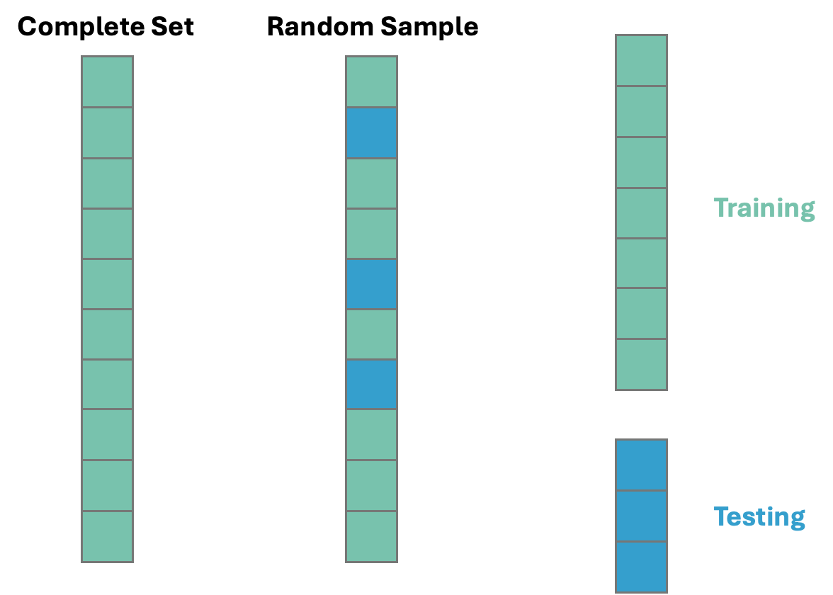
Before exploring any relationships between predictor variables and the target variable SalePrice, we need to split our data set into training and testing pieces. Because models are prone to discovering small, spurious patterns on the data that is used to create them (the training data), we set aside the testing data to get a clear view of how they might perform on new data that the models have never seen before.
from sklearn.model_selection import train_test_split
train, test = train_test_split(ames, test_size = 0.25, random_state = 1234)This split is done randomly. However, to make sure we can replicate this random split we use the random_state option. The data is split randomly so that the testing data set will approximate an honest assessment of how the model will perform in a real world setting. A visual representation of this is below:
Once we have our data split into training and testing datasets, we can now start to explore the relationships in the training data.
Before we start fully exploring our data we can now finish handling our missing values. We should not replace continuous predictor variable missing values on the whole dataset because that would impute the mean/median of the whole variable, not just the training data. We are not allowed to run any analysis on the whole dataset. This is especially the case if you wanted to impute missing values of a continuous variable using other variables in the dataset.
Let’s do this in each software!
The missing values from categorical predictor variables have already been imputed with a new category called Missing in the previous section. Therefore, we need to only look at the continuous variables for imputation at this stage. We isolate those variables using the select_dtypes function with the include = numeric option as well as the columns function.
num_cols = train.select_dtypes(include = 'number').columnsNow that we have a list of columns that are numerical in type we can loop through that list using a for loop. We identify any column that has missing values using the isnull and any functions after an if statement. Next, we create a missing value flag for that those columns in the loop based on the name of the variable using the isnull function. To convert these to the integer values of 0 and 1 we convert the type with the astype(int) function on that new variable. Lastly, we calculate the median of the variable of interest using the median function and then take that median calculation and put it in the fillna function to replace all the missing values in the variable. The loop continues this calculation for the rest of the variables.
for col in num_cols:
    if train[col].isnull().any():
        # Create missing flag column
        train[f'{col}_was_missing'] = train[col].isnull().astype(int)

        # Impute with median
        median = train[col].median()
        train[col] = train[col].fillna(median)
Now our data is ready to explore!
To make sure we are getting the same data to analyze in R, we will import the Python train and test datasets. However, something similar can be done in R using the sample_frac function from the tidyverse package using the following code:
library(tidyverse)

ames <- ames %>% mutate(id = row_number())

set.seed(4321)

training <- ames %>% sample_frac(0.7)
testing <- anti_join(ames, training, by = 'id')
Again, the above code was not run. The train and test datasets from Python were imported to make the analysis comparable.
train <- py$train
test <- py$test
The missing values from categorical predictor variables have already been imputed with a new category called Missing in the previous section. Therefore, we need to only look at the continuous variables for imputation at this stage. We isolate those variables using the sapply function with the is,numeric function within it.
num_cols <- names(train)[sapply(train, is.numeric)]Now that we have a list of columns that are numerical in type we can loop through that list using a for loop. We identify any column that has missing values using the is.na and any functions after an if statement. Next, we create a missing value flag for that those columns in the loop based on the name of the variable using the paste0 function. To convert these to the integer values of 0 and 1 we convert the type with the as.integer function on the variables identified with the is.na function. Lastly, we calculate the median of the variable of interest using the median function and then take that median calculation and put it in the is.na function with specific double [[ and ]] to replace all the missing values in the variable. The loop continues this calculation for the rest of the variables.
for (col in num_cols) {
  if (any(is.na(train[[col]]))) {

    # Create a missing flag column
    flag_col <- paste0(col, "_was_missing")
    train[[flag_col]] <- as.integer(is.na(train[[col]]))

    # Impute with median
    median_value <- median(train[[col]], na.rm = TRUE)
    train[[col]][is.na(train[[col]])] <- median_value
  }
}
Now our data is ready to explore!
Once we have data that is ready to explore relationships we can quickly explore some individual predictor variable relationships with our target variable. If we have a small list of variables, this can be done by looking over scatterplots between your continuous predictor variables and your continuous target and boxplots for categorical predictors variables with your continuous target. However, when the list of variables starts to get large this becomes a burden. In these scenarios we can use automated techniques to quickly evaluate basic relationships between our predictors and our target. A quick word of caution; any time you use automated techniques to quickly go through large lists of variables, there is a chance that a couple of variables with really complicated relationships might slip through these simple relationship screenings. We are hoping that the large number of variables will overcome this problem and we are left with a large number still to pick from. That is why with smaller numbers of variables, visual exploration is always preferred.
The approach we will take is to look at univariate statistical tests between one predictor variable at a time with our target variable. We will screen out variables with p-values that are too high. Initial p-value selection is a common approach to remove variables with very low linear predictive power with our continuous target variable. The cut-off for these p-values is a critical question. A lot of introductory statistical test use a cut-off of 0.05. Anything below that would be considered statistically significant and worth moving on to the next stage of model building. However, this is a common misconception. The original author of the p-value, hypothesis test approach used 0.05 for their sample sizes of 50. It has been shown since that larger sample sizes need far lower cut-offs (referred to as \(\alpha\)-levels) to be reasonable. These \(\alpha\)-levels correspond to the probability of making a Type I error - in our scenario, falsely thinking a variable is significant when it really is not.
In a paper from 1994, Raftery provides more reasonable \(\alpha\)-levels based on sample size of the training dataset:
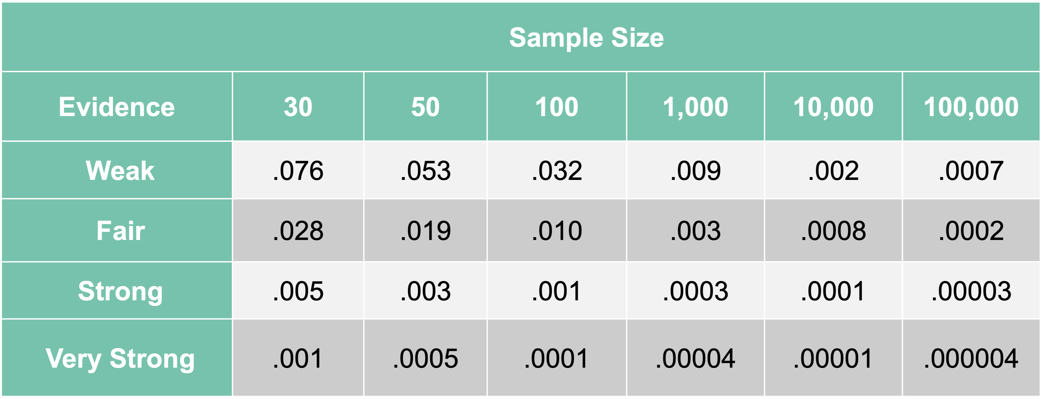
As we can see, an \(\alpha\)-level of 0.05 is good for sample sizes of about 50 for finding weak relationships. For the sample size of our data, a cut-off of about 0.009 is much more reasonable. We still want to find anything with at least a weak relationship with our target since we don’t want to be too restrictive this early on.
The p-value we use comes from the F-test from a simple linear regression. We will compare each individual variable in a simple linear regression with our target variable and record the F statistic p-value. The F-statistic is calculated as:
\[ F = \frac{MSR}{MSE} \]
where \(MSR\) refers to the mean square calculation from the regression model and \(MSE\) refers to the mean square calculation from the errors. More formally, \(MSR\) is the variance that is explained by the regression model. This is calculated by comparing the predictions from the regression model, \(\hat{y}_i\), to the overall average prediction, \(\bar{y}\):
\[ SSR = \sum_{i=1}^n (\hat{y}_i - \bar{y})^2 \]
This \(SSR\) is then divided by how many variables we have in the model, \(p\). In our scenario, \(p=1\). This can be thought of as the “average” of the variance explained per variable in the model.
This is then compared to the \(MSE\). The \(MSE\) is the variance that is unexplained from the model. This is calculated by comparing the true values of our target variable, \(y_i\), to our regression model’s predictions, \(\hat{y}_i\):
\[ SSE = \sum_{i=1}^n (y_i - \hat{y}_i)^2 \]
This \(SSE\) is then divided by the degrees of freedom in our error: \(n-p-1\). This can be thought of as the “average” amount of the remaining, unexplained variance per observation left over from our model.
Combining these together gives us our original F statistic:
\[ F = \frac{MSR}{MSE} = \frac{SSR/p}{SSE/(n-p-1)} \]
This ratio compares the amount of variation our model was able to explain (per variable) to how much variation is still left over (per observation). The more our model can explain, the larger this ratio becomes, which then makes our p-value smaller.
Let’s look at these automated approaches in each software!
Before we can put the predictor variables in our functions for automated screening we need to convert our categorical variables into dummy coded variables. Essentially, we need to one-hot encode our variables to make each category have a corresponding binary flag variable. Using the get_dummies function from Pandas we can do this easily. First, we must remove the target variable from our training data with the drop function. Just to make sure that all variables are of the same type, after converting the variables to binary flags we use the astype(float) function on all our predictor variables. Lastly, we call the predictor variables dataframe X and our target variable y.
import statsmodels.api as sm

# Dummy Code the Categorical Variables
predictors = train.drop(columns = ['SalePrice'])
predictors = pd.get_dummies(predictors, drop_first = True)
predictors = predictors.astype(float)

# Create Predictor and Target Objects
X = predictors
y = train['SalePrice']
Once our data is in this format we can use the SelectKBest and f_regression functions from the popular sci-kit learn package, specifically sklearn.feature_selection. Inside SelectKBest we will use the f_regression function as our scoring function for each of the predictor variables. There are other options for a classification target if we had that instead. The k = 'all' option doesn’t eliminate any variables, but instead calculates the p-value for each variable. That way we can be the ones to decide which variables we want to keep. We then input our X and y objects into the fit function on the SelectKBest object. From there we just save the column names (columns), the test statistics (scores_), and p-values (pvalues_) into a single dataframe. We then use sort_values to sort in descending order by the F-statistic followed by printing them out to view.
from sklearn.feature_selection import SelectKBest, f_regression

# Fit SelectKBest but Show ALL Variables
selector = SelectKBest(score_func = f_regression, k = 'all')
selector.fit(X, y)
SelectKBest(k='all', score_func=<function f_regression at 0x32ee92840>)In a Jupyter environment, please rerun this cell to show the HTML representation or trust the notebook.
| score_func | <function f_r...t 0x32ee92840> | |
| k | 'all' |
# Create a DataFrame with feature names, F-scores, and p-values
scores_df = pd.DataFrame({
    'Feature': X.columns,
    'F_score': selector.scores_,
    'p_value': selector.pvalues_
})

# Sort by F-score descending
scores_df = scores_df.sort_values(by = 'F_score', ascending = False)

with pd.option_context('display.max_rows', None):
    print(scores_df)
Feature F_score p_value
2 OverallQual 1797.933303 4.305605e-233
8 GrLivArea 1083.918902 1.020195e-165
15 GarageCars 765.779731 3.526828e-128
16 GarageArea 679.101741 7.889357e-117
5 TotalBsmtSF 646.873094 1.818769e-112
6 1stFlrSF 640.245441 1.468943e-111
59 ExterQual_TA 555.825075 1.091141e-99
9 FullBath 477.720517 3.783999e-88
12 TotRmsAbvGrd 441.455145 1.361562e-82
76 KitchenQual_TA 402.015773 2.131390e-76
3 YearBuilt 386.023126 7.721397e-74
4 YearRemodAdd 381.849868 3.631354e-73
61 Foundation_PConc 375.129664 4.434457e-72
79 FireplaceQu_Missing 319.568158 6.755886e-63
13 Fireplaces 306.200382 1.240533e-60
14 GarageYrBlt 301.858406 6.818288e-60
68 BsmtQual_TA 275.524512 2.359938e-55
58 ExterQual_Gd 272.465749 8.051814e-55
86 GarageType_Detchd 168.736149 5.539706e-36
60 Foundation_CBlock 164.079394 4.229420e-35
82 GarageType_Attchd 151.637635 1.004137e-32
78 FireplaceQu_Gd 146.811156 8.512176e-32
0 LotFrontage 128.797978 2.682367e-28
18 OpenPorchSF 126.262795 8.419876e-28
7 2ndFlrSF 123.006569 3.672964e-27
72 HeatingQC_TA 119.599354 1.723333e-26
75 KitchenQual_Gd 114.516225 1.744797e-25
17 WoodDeckSF 111.941158 5.659995e-25
10 HalfBath 91.719347 6.435196e-21
30 LotShape_Reg 90.973468 9.112442e-21
1 LotArea 89.357988 1.937363e-20
97 GarageCond_TA 77.303445 5.596804e-18
54 HouseStyle_2Story 65.162272 1.806906e-15
73 CentralAir_Y 61.719648 9.424915e-15
84 GarageType_BuiltIn 57.950794 5.790911e-14
92 GarageQual_TA 57.457470 7.348571e-14
99 PavedDrive_Y 56.673698 1.073223e-13
87 GarageType_Missing 50.790290 1.863241e-12
95 GarageCond_Missing 50.790290 1.863241e-12
90 GarageQual_Missing 50.790290 1.863241e-12
27 GarageYrBlt_was_missing 50.790290 1.863241e-12
66 BsmtQual_Gd 49.776415 3.053328e-12
11 BedroomAbvGr 30.079500 5.149951e-08
74 KitchenQual_Fa 27.614571 1.779402e-07
67 BsmtQual_Missing 25.341035 5.614454e-07
34 LotConfig_CulDSac 25.236681 5.919311e-07
81 FireplaceQu_TA 24.333809 9.357904e-07
70 HeatingQC_Gd 23.388627 1.513049e-06
28 LotShape_IR2 21.719834 3.543780e-06
88 GarageQual_Fa 20.771390 5.757747e-06
93 GarageCond_Fa 18.677569 1.688980e-05
65 BsmtQual_Fa 18.280909 2.072552e-05
62 Foundation_Slab 17.987483 2.411733e-05
21 ScreenPorch 16.235861 5.979623e-05
19 EnclosedPorch 15.681304 7.981091e-05
47 BldgType_Duplex 15.621239 8.234931e-05
31 LandContour_HLS 15.582714 8.402011e-05
69 HeatingQC_Fa 15.385770 9.311052e-05
38 Condition1_Feedr 15.134336 1.061724e-04
57 ExterQual_Fa 14.806939 1.259915e-04
39 Condition1_Norm 13.551221 2.434765e-04
22 PoolArea 13.321565 2.747717e-04
48 BldgType_Twnhs 11.867634 5.928564e-04
50 HouseStyle_1.5Unf 11.011222 9.354708e-04
55 HouseStyle_SFoyer 10.087611 1.534472e-03
46 BldgType_2fmCon 9.241976 2.421586e-03
37 LotConfig_Inside 8.929279 2.869035e-03
98 PavedDrive_P 7.166567 7.538699e-03
85 GarageType_CarPort 7.156097 7.582535e-03
80 FireplaceQu_Po 5.439181 1.987078e-02
96 GarageCond_Po 4.885545 2.728904e-02
56 HouseStyle_SLvl 4.417574 3.579898e-02
42 Condition1_RRAe 3.376259 6.641335e-02
52 HouseStyle_2.5Fin 3.309407 6.915784e-02
91 GarageQual_Po 3.044455 8.129434e-02
89 GarageQual_Gd 2.364968 1.243759e-01
40 Condition1_PosA 2.253958 1.335620e-01
51 HouseStyle_1Story 2.245865 1.342607e-01
41 Condition1_PosN 1.984733 1.591771e-01
32 LandContour_Low 1.774032 1.831615e-01
83 GarageType_Basment 1.575615 2.096617e-01
20 3SsnPorch 1.496580 2.214620e-01
24 MoSold 1.415675 2.343749e-01
71 HeatingQC_Po 1.360606 2.436870e-01
25 YrSold 0.923403 3.367957e-01
53 HouseStyle_2.5Unf 0.900878 3.427561e-01
77 FireplaceQu_Fa 0.695147 4.046014e-01
45 Condition1_RRNn 0.666911 4.143088e-01
23 MiscVal 0.442107 5.062475e-01
36 LotConfig_FR3 0.402045 5.261676e-01
33 LandContour_Lvl 0.250091 6.171118e-01
63 Foundation_Stone 0.246604 6.195765e-01
26 LotFrontage_was_missing 0.222654 6.371196e-01
43 Condition1_RRAn 0.168449 6.815742e-01
29 LotShape_IR3 0.112438 7.374501e-01
94 GarageCond_Gd 0.091308 7.625783e-01
49 BldgType_TwnhsE 0.078756 7.790435e-01
35 LotConfig_FR2 0.005812 9.392463e-01
64 Foundation_Wood 0.004392 9.471704e-01
44 Condition1_RRNe 0.002970 9.565476e-01We now have a list of variables by their respective F-statistics and p-values. The OverallQual variable seems to be the most predictive.
From here we can remove the variables with a p-value above our 0.009 cut-off by isolating the specific variables that meet that requirement. We then select only those variables from our original X object to get our reduced variable list called X_reduced.
# Filter for features with p-value < 0.009
selected_features = scores_df[scores_df['p_value'] < 0.009]['Feature']

# Create a new DataFrame with only those selected columns
X_reduced = X[selected_features.tolist()]
Before we can put the predictor variables in our functions for automated screening we need to convert our categorical variables into dummy coded variables. Essentially, we need to one-hot encode our variables to make each category have a corresponding binary flag variable. Using the model.matrix function we can do this easily. First, we must remove the target variable from our training data with the select function. Lastly, we call the predictor variables dataframe X and our target variable y.
library(broom)
library(dplyr)

# Create Predictor and Target Objects
y <- train$SalePrice
predictors <- train %>% select(-SalePrice)

# Dummy Code the Categorical Variables
X <- model.matrix(~ . - 1, data = predictors) %>% as.data.frame()

names(X)[names(X) == "`1stFlrSF`"] <- "FirstFlrSF"
names(X)[names(X) == "`2ndFlrSF`"] <- "SecondFlrSF"
names(X)[names(X) == "`3SsnPorch`"] <- "ThreeStoryPorch"
Once our data is in this format we can use the lapply function and input our own function where we calculate the individual linear regressions. We will create our own function called feat where we calculate individual linear regressions with the lm function. From those individual regressions we use the summary function to extract the F-statistic information. From that information we can calculate the p-value using the pf function with the lower.tail = FALSE option. This approach doesn’t eliminate any variables, but instead calculates the p-value for each variable. That way we can be the ones to decide which variables we want to keep. We then use bind_rows to combine the information into a single data frame where we use desc to sort in descending order by the F-statistic followed by printing them out to view.
# Store feature names
features <- names(X)

# Loop through each feature, run univariate linear regression, and sort
scores_df <- lapply(features, function(feat) {
  model <- lm(as.formula(paste("y ~", feat)), data = cbind(y = y, X))
  f_val <- summary(model)$fstatistic
  data.frame(
    Feature = feat,
    F_score = f_val[1],
    p_value = pf(f_val[1], f_val[2], f_val[3], lower.tail = FALSE)
  )
}) %>% bind_rows() %>%
  arrange(desc(F_score))

# Print final result
print(scores_df)
Feature F_score p_value
value...1 OverallQual 1.797933e+03 4.305605e-233
value...2 GrLivArea 1.083919e+03 1.020195e-165
value...3 GarageCars 7.657797e+02 3.526828e-128
value...4 GarageArea 6.791017e+02 7.889357e-117
value...5 TotalBsmtSF 6.468731e+02 1.818769e-112
value...6 FirstFlrSF 6.402454e+02 1.468943e-111
value...7 ExterQualTA 5.558251e+02 1.091141e-99
value...8 FullBath 4.777205e+02 3.783999e-88
value...9 TotRmsAbvGrd 4.414551e+02 1.361562e-82
value...10 KitchenQualTA 4.020158e+02 2.131390e-76
value...11 YearBuilt 3.860231e+02 7.721397e-74
value...12 YearRemodAdd 3.818499e+02 3.631354e-73
value...13 FoundationPConc 3.751297e+02 4.434457e-72
value...14 FireplaceQuMissing 3.195682e+02 6.755886e-63
value...15 Fireplaces 3.062004e+02 1.240533e-60
value...16 GarageYrBlt 3.018584e+02 6.818288e-60
value...17 BsmtQualTA 2.755245e+02 2.359938e-55
value...18 ExterQualGd 2.724657e+02 8.051814e-55
value...19 GarageTypeDetchd 1.687361e+02 5.539706e-36
value...20 FoundationCBlock 1.640794e+02 4.229420e-35
value...21 GarageTypeAttchd 1.516376e+02 1.004137e-32
value...22 FireplaceQuGd 1.468112e+02 8.512176e-32
value...23 LotFrontage 1.287980e+02 2.682367e-28
value...24 OpenPorchSF 1.262628e+02 8.419876e-28
value...25 SecondFlrSF 1.230066e+02 3.672964e-27
value...26 HeatingQCTA 1.195994e+02 1.723333e-26
value...27 KitchenQualGd 1.145162e+02 1.744797e-25
value...28 WoodDeckSF 1.119412e+02 5.659995e-25
value...29 HalfBath 9.171935e+01 6.435196e-21
value...30 LotShapeReg 9.097347e+01 9.112442e-21
value...31 LotArea 8.935799e+01 1.937363e-20
value...32 GarageCondTA 7.730344e+01 5.596804e-18
value...33 HouseStyle2Story 6.516227e+01 1.806906e-15
value...34 LotShapeIR1 6.189296e+01 8.671583e-15
value...35 CentralAirY 6.171965e+01 9.424915e-15
value...36 GarageTypeBuiltIn 5.795079e+01 5.790911e-14
value...37 GarageQualTA 5.745747e+01 7.348571e-14
value...38 PavedDriveY 5.667370e+01 1.073223e-13
value...39 GarageTypeMissing 5.079029e+01 1.863241e-12
value...40 GarageQualMissing 5.079029e+01 1.863241e-12
value...41 GarageCondMissing 5.079029e+01 1.863241e-12
value...42 GarageYrBlt_was_missing 5.079029e+01 1.863241e-12
value...43 BsmtQualGd 4.977642e+01 3.053328e-12
value...44 BedroomAbvGr 3.007950e+01 5.149951e-08
value...45 KitchenQualFa 2.761457e+01 1.779402e-07
value...46 BsmtQualMissing 2.534103e+01 5.614454e-07
value...47 LotConfigCulDSac 2.523668e+01 5.919311e-07
value...48 FireplaceQuTA 2.433381e+01 9.357904e-07
value...49 HeatingQCGd 2.338863e+01 1.513049e-06
value...50 LotShapeIR2 2.171983e+01 3.543780e-06
value...51 GarageQualFa 2.077139e+01 5.757747e-06
value...52 GarageCondFa 1.867757e+01 1.688980e-05
value...53 BsmtQualFa 1.828091e+01 2.072552e-05
value...54 FoundationSlab 1.798748e+01 2.411733e-05
value...55 ScreenPorch 1.623586e+01 5.979623e-05
value...56 EnclosedPorch 1.568130e+01 7.981091e-05
value...57 BldgTypeDuplex 1.562124e+01 8.234931e-05
value...58 LandContourHLS 1.558271e+01 8.402011e-05
value...59 HeatingQCFa 1.538577e+01 9.311052e-05
value...60 Condition1Feedr 1.513434e+01 1.061724e-04
value...61 ExterQualFa 1.480694e+01 1.259915e-04
value...62 Condition1Norm 1.355122e+01 2.434765e-04
value...63 PoolArea 1.332157e+01 2.747717e-04
value...64 BldgTypeTwnhs 1.186763e+01 5.928564e-04
value...65 HouseStyle1.5Unf 1.101122e+01 9.354708e-04
value...66 HouseStyleSFoyer 1.008761e+01 1.534472e-03
value...67 BldgType2fmCon 9.241976e+00 2.421586e-03
value...68 LotConfigInside 8.929279e+00 2.869035e-03
value...69 PavedDriveP 7.166567e+00 7.538699e-03
value...70 GarageTypeCarPort 7.156097e+00 7.582535e-03
value...71 FireplaceQuPo 5.439181e+00 1.987078e-02
value...72 GarageCondPo 4.885545e+00 2.728904e-02
value...73 HouseStyleSLvl 4.417574e+00 3.579898e-02
value...74 Condition1RRAe 3.376259e+00 6.641335e-02
value...75 HouseStyle2.5Fin 3.309407e+00 6.915784e-02
value...76 GarageQualPo 3.044455e+00 8.129434e-02
value...77 GarageQualGd 2.364968e+00 1.243759e-01
value...78 Condition1PosA 2.253958e+00 1.335620e-01
value...79 HouseStyle1Story 2.245865e+00 1.342607e-01
value...80 Condition1PosN 1.984733e+00 1.591771e-01
value...81 LandContourLow 1.774032e+00 1.831615e-01
value...82 GarageTypeBasment 1.575615e+00 2.096617e-01
value...83 ThreeStoryPorch 1.496580e+00 2.214620e-01
value...84 MoSold 1.415675e+00 2.343749e-01
value...85 HeatingQCPo 1.360606e+00 2.436870e-01
value...86 YrSold 9.234026e-01 3.367957e-01
value...87 HouseStyle2.5Unf 9.008783e-01 3.427561e-01
value...88 FireplaceQuFa 6.951470e-01 4.046014e-01
value...89 Condition1RRNn 6.669105e-01 4.143088e-01
value...90 MiscVal 4.421070e-01 5.062475e-01
value...91 LotConfigFR3 4.020451e-01 5.261676e-01
value...92 LandContourLvl 2.500908e-01 6.171118e-01
value...93 FoundationStone 2.466039e-01 6.195765e-01
value...94 LotFrontage_was_missing 2.226536e-01 6.371196e-01
value...95 Condition1RRAn 1.684491e-01 6.815742e-01
value...96 LotShapeIR3 1.124377e-01 7.374501e-01
value...97 GarageCondGd 9.130802e-02 7.625783e-01
value...98 BldgTypeTwnhsE 7.875602e-02 7.790435e-01
value...99 LotConfigFR2 5.811741e-03 9.392463e-01
value...100 FoundationWood 4.392474e-03 9.471704e-01
value...101 Condition1RRNe 2.970138e-03 9.565476e-01We now have a list of variables by their respective F-statistics and p-values. The OverallQual variable seems to be the most predictive.
From here we can remove the variables with a p-value above our 0.009 cut-off by isolating the specific variables that meet that requirement. We then select only those variables from our original X object to get our reduced variable list called X_reduced.
# Filter for features with p-value < 0.009
selected_features <- scores_df %>%
  filter(p_value < 0.009) %>%
  pull(Feature)

# Create a new data frame with only those selected columns
X_reduced <- X[, selected_features, drop = FALSE]Now we have a reduced list of variables from our data exploration. Before diving into model building concepts let’s build an initial model at our current state.
Now that we have a shorter variable list, let’s build an initial multiple linear regression model:
\[ \hat{y}_i = \hat{\beta}_0 + \hat{\beta}_1 x_{1,i} + \cdots + \hat{\beta}_p x_{p,i} \]
Once we take a look at this initial linear regression, then we will evaluate which variables we want to keep.
Let’s see how to do this in each of our software!
Before building a model in Python using the statsmodels.api package, we need to add a column of all 1’s. This column of all 1’s will create the intercept term, \(\beta_0\), in the linear regression. To do this we use the add_constant function on our reduced predictor variable dataframe. From there we just input the target variable and our predictor variables into the OLS function from statsmodels.api. The fit function will then fit our respective linear regression. Lastly, we use the summary function to view the output.
import statsmodels.api as sm

X_reduced = sm.add_constant(X_reduced)
model = sm.OLS(y, X_reduced)
result = model.fit()

print(result.summary())
OLS Regression Results
==============================================================================
Dep. Variable: SalePrice R-squared: 0.829
Model: OLS Adj. R-squared: 0.818
Method: Least Squares F-statistic: 75.26
Date: Sat, 15 Nov 2025 Prob (F-statistic): 0.00
Time: 10:50:47 Log-Likelihood: -12977.
No. Observations: 1095 AIC: 2.609e+04
Df Residuals: 1028 BIC: 2.642e+04
Df Model: 66
Covariance Type: nonrobust
===========================================================================================
coef std err t P>|t| [0.025 0.975]
-------------------------------------------------------------------------------------------
const -8.745e+04 2.54e+05 -0.344 0.731 -5.86e+05 4.11e+05
OverallQual 1.243e+04 1529.620 8.126 0.000 9427.513 1.54e+04
GrLivArea 1.0898 23.844 0.046 0.964 -45.699 47.879
GarageCars 1.339e+04 3624.893 3.694 0.000 6276.531 2.05e+04
GarageArea 25.8692 11.854 2.182 0.029 2.609 49.129
TotalBsmtSF 13.2116 6.415 2.059 0.040 0.623 25.800
1stFlrSF 37.1809 24.551 1.514 0.130 -10.994 85.356
ExterQual_TA -1.643e+04 8375.482 -1.961 0.050 -3.29e+04 9.692
FullBath 2177.6897 3377.463 0.645 0.519 -4449.820 8805.199
TotRmsAbvGrd 2150.1420 1458.739 1.474 0.141 -712.304 5012.588
KitchenQual_TA -3.76e+04 6384.526 -5.890 0.000 -5.01e+04 -2.51e+04
YearBuilt 183.5406 99.159 1.851 0.064 -11.036 378.117
YearRemodAdd 136.7789 83.252 1.643 0.101 -26.585 300.143
Foundation_PConc 1.391e+04 5578.347 2.494 0.013 2968.437 2.49e+04
FireplaceQu_Missing 2719.7438 7145.154 0.381 0.704 -1.13e+04 1.67e+04
Fireplaces 1.127e+04 4350.193 2.592 0.010 2738.713 1.98e+04
GarageYrBlt -261.6592 92.929 -2.816 0.005 -444.012 -79.306
BsmtQual_TA -3.679e+04 6601.991 -5.573 0.000 -4.97e+04 -2.38e+04
ExterQual_Gd -1.173e+04 7482.799 -1.568 0.117 -2.64e+04 2953.250
GarageType_Detchd 9558.9692 9097.893 1.051 0.294 -8293.592 2.74e+04
Foundation_CBlock 1.342e+04 4979.062 2.695 0.007 3648.407 2.32e+04
GarageType_Attchd 1.226e+04 8993.147 1.363 0.173 -5387.657 2.99e+04
FireplaceQu_Gd -7087.3241 5448.909 -1.301 0.194 -1.78e+04 3604.929
LotFrontage -35.6152 62.515 -0.570 0.569 -158.287 87.056
OpenPorchSF -17.6777 17.953 -0.985 0.325 -52.906 17.551
2ndFlrSF 53.1360 24.650 2.156 0.031 4.765 101.507
HeatingQC_TA -6243.5810 3274.991 -1.906 0.057 -1.27e+04 182.849
KitchenQual_Gd -3.022e+04 5638.921 -5.360 0.000 -4.13e+04 -1.92e+04
WoodDeckSF 33.4070 9.319 3.585 0.000 15.120 51.694
HalfBath 919.7145 3260.459 0.282 0.778 -5478.201 7317.630
LotShape_Reg -3858.9488 2546.583 -1.515 0.130 -8856.043 1138.145
LotArea 0.1977 0.142 1.395 0.163 -0.080 0.476
GarageCond_TA 1.133e+04 1.11e+04 1.021 0.307 -1.04e+04 3.31e+04
HouseStyle_2Story -1.476e+04 4711.293 -3.133 0.002 -2.4e+04 -5516.886
CentralAir_Y 2660.7298 5988.337 0.444 0.657 -9090.031 1.44e+04
GarageType_BuiltIn 1.077e+04 1.04e+04 1.033 0.302 -9691.479 3.12e+04
GarageQual_TA -1.946e+04 1.05e+04 -1.853 0.064 -4.01e+04 1151.166
PavedDrive_Y 3224.5206 5564.756 0.579 0.562 -7695.056 1.41e+04
GarageType_Missing 8484.6693 3962.121 2.141 0.032 709.900 1.63e+04
GarageCond_Missing 8484.6693 3962.121 2.141 0.032 709.900 1.63e+04
GarageQual_Missing 8484.6693 3962.121 2.141 0.032 709.900 1.63e+04
GarageYrBlt_was_missing 8484.6693 3962.121 2.141 0.032 709.900 1.63e+04
BsmtQual_Gd -3.593e+04 5316.082 -6.758 0.000 -4.64e+04 -2.55e+04
BedroomAbvGr -1692.3586 2087.286 -0.811 0.418 -5788.186 2403.468
KitchenQual_Fa -3.751e+04 9832.196 -3.815 0.000 -5.68e+04 -1.82e+04
BsmtQual_Missing -2.512e+04 1.66e+04 -1.513 0.131 -5.77e+04 7458.243
LotConfig_CulDSac 1.241e+04 5473.956 2.266 0.024 1664.626 2.31e+04
FireplaceQu_TA -5272.0765 5524.834 -0.954 0.340 -1.61e+04 5569.164
HeatingQC_Gd -4929.1065 3348.159 -1.472 0.141 -1.15e+04 1640.900
LotShape_IR2 1.384e+04 6924.985 1.998 0.046 249.567 2.74e+04
GarageQual_Fa -2.549e+04 1.2e+04 -2.123 0.034 -4.9e+04 -1933.388
GarageCond_Fa 1.142e+04 1.3e+04 0.875 0.382 -1.42e+04 3.7e+04
BsmtQual_Fa -4.171e+04 9989.190 -4.176 0.000 -6.13e+04 -2.21e+04
Foundation_Slab 2737.4065 1.71e+04 0.160 0.873 -3.07e+04 3.62e+04
ScreenPorch 56.4523 19.636 2.875 0.004 17.921 94.983
EnclosedPorch 4.4598 19.374 0.230 0.818 -33.557 42.476
BldgType_Duplex -2.193e+04 7500.892 -2.924 0.004 -3.66e+04 -7212.060
LandContour_HLS 6639.3386 6447.555 1.030 0.303 -6012.533 1.93e+04
HeatingQC_Fa -2907.5365 7307.787 -0.398 0.691 -1.72e+04 1.14e+04
Condition1_Feedr -987.5563 6084.564 -0.162 0.871 -1.29e+04 1.1e+04
ExterQual_Fa -2.059e+04 1.46e+04 -1.411 0.159 -4.92e+04 8049.064
Condition1_Norm 1.247e+04 4066.459 3.068 0.002 4495.034 2.05e+04
PoolArea -76.3474 32.180 -2.373 0.018 -139.493 -13.202
BldgType_Twnhs -1.906e+04 7258.792 -2.626 0.009 -3.33e+04 -4820.314
HouseStyle_1.5Unf 5347.2965 1.04e+04 0.513 0.608 -1.51e+04 2.58e+04
HouseStyle_SFoyer 3841.6662 8117.844 0.473 0.636 -1.21e+04 1.98e+04
BldgType_2fmCon -1.267e+04 8102.544 -1.564 0.118 -2.86e+04 3230.109
LotConfig_Inside -600.4065 2769.771 -0.217 0.828 -6035.456 4834.643
PavedDrive_P 1252.2416 9240.160 0.136 0.892 -1.69e+04 1.94e+04
GarageType_CarPort 5815.4725 1.54e+04 0.378 0.705 -2.43e+04 3.6e+04
==============================================================================
Omnibus: 431.767 Durbin-Watson: 2.057
Prob(Omnibus): 0.000 Jarque-Bera (JB): 50780.630
Skew: -0.779 Prob(JB): 0.00
Kurtosis: 36.325 Cond. No. 1.28e+16
==============================================================================
Notes:
[1] Standard Errors assume that the covariance matrix of the errors is correctly specified.
[2] The smallest eigenvalue is 1.4e-21. This might indicate that there are
strong multicollinearity problems or that the design matrix is singular.We can see that we still have a lot of variables left in out regression model. Even though individually those predictor variables were all significant, together that is no longer the case. In the next section we will discuss strategies to help reduce the variable list even further.
In R we just input the target variable and our predictor variables into the lm function using the formula framework. Here, having the formula y ~ . uses our defined target variable object y we defined earlier and all of the variables in the X_reduced dataframe. Lastly, we use the summary function to view the output.
model <- lm(y ~ ., data = X_reduced)

summary(model)
Call:
lm(formula = y ~ ., data = X_reduced)

Residuals:
    Min      1Q  Median      3Q     Max
-346458  -14779     399   13884  270746

Coefficients: (3 not defined because of singularities)
                          Estimate Std. Error t value Pr(>|t|)
(Intercept)             -2.708e+05  2.527e+05  -1.071 0.284205
OverallQual              1.236e+04  1.509e+03   8.189 7.78e-16 ***
GrLivArea                1.218e+00  2.352e+01   0.052 0.958700
GarageCars               1.213e+04  3.583e+03   3.387 0.000735 ***
GarageArea               2.733e+01  1.170e+01   2.337 0.019623 *
TotalBsmtSF              1.694e+01  6.365e+00   2.661 0.007922 **
FirstFlrSF               3.743e+01  2.422e+01   1.546 0.122510
ExterQualTA             -1.770e+04  8.265e+03  -2.142 0.032451 *
FullBath                 1.347e+03  3.335e+03   0.404 0.686294
TotRmsAbvGrd             1.653e+03  1.442e+03   1.146 0.251871
KitchenQualTA           -3.607e+04  6.304e+03  -5.721 1.39e-08 ***
YearBuilt                1.922e+02  9.783e+01   1.965 0.049660 *
YearRemodAdd             1.572e+02  8.221e+01   1.912 0.056188 .
FoundationPConc          1.274e+04  5.507e+03   2.313 0.020907 *
FireplaceQuMissing       1.992e+03  7.050e+03   0.283 0.777602
Fireplaces               1.162e+04  4.292e+03   2.708 0.006880 **
GarageYrBlt             -2.428e+02  9.173e+01  -2.647 0.008257 **
BsmtQualTA              -3.441e+04  6.527e+03  -5.272 1.65e-07 ***
ExterQualGd             -1.296e+04  7.385e+03  -1.755 0.079565 .
GarageTypeDetchd         9.835e+03  8.975e+03   1.096 0.273375
FoundationCBlock         1.159e+04  4.923e+03   2.354 0.018783 *
GarageTypeAttchd         1.173e+04  8.872e+03   1.322 0.186359
FireplaceQuGd           -7.917e+03  5.377e+03  -1.472 0.141237
LotFrontage              7.495e+00  6.218e+01   0.121 0.904081
OpenPorchSF             -2.093e+01  1.772e+01  -1.181 0.237904
SecondFlrSF              5.415e+01  2.432e+01   2.227 0.026186 *
HeatingQCTA             -6.312e+03  3.231e+03  -1.954 0.051011 .
KitchenQualGd           -2.924e+04  5.565e+03  -5.255 1.80e-07 ***
WoodDeckSF               3.423e+01  9.194e+00   3.723 0.000207 ***
HalfBath                 6.860e+02  3.217e+03   0.213 0.831153
LotShapeReg              8.535e+04  1.663e+04   5.134 3.40e-07 ***
LotArea                  2.232e-01  1.400e-01   1.595 0.111092
GarageCondTA             1.211e+04  1.094e+04   1.107 0.268597
HouseStyle2Story        -1.379e+04  4.651e+03  -2.964 0.003102 **
LotShapeIR1              9.014e+04  1.661e+04   5.428 7.11e-08 ***
CentralAirY              3.942e+02  5.922e+03   0.067 0.946937
GarageTypeBuiltIn        1.217e+04  1.029e+04   1.183 0.237129
GarageQualTA            -1.884e+04  1.036e+04  -1.818 0.069354 .
PavedDriveY              1.764e+03  5.496e+03   0.321 0.748260
GarageTypeMissing        3.350e+04  1.563e+04   2.143 0.032349 *
GarageQualMissing               NA         NA      NA       NA
GarageCondMissing               NA         NA      NA       NA
GarageYrBlt_was_missing         NA         NA      NA       NA
BsmtQualGd              -3.394e+04  5.257e+03  -6.456 1.66e-10 ***
BedroomAbvGr            -1.598e+03  2.059e+03  -0.776 0.437822
KitchenQualFa           -3.712e+04  9.699e+03  -3.827 0.000138 ***
BsmtQualMissing         -2.031e+04  1.640e+04  -1.238 0.215872
LotConfigCulDSac         1.192e+04  5.400e+03   2.208 0.027461 *
FireplaceQuTA           -6.296e+03  5.453e+03  -1.155 0.248530
HeatingQCGd             -4.509e+03  3.304e+03  -1.365 0.172613
LotShapeIR2              1.022e+05  1.765e+04   5.789 9.39e-09 ***
GarageQualFa            -2.503e+04  1.184e+04  -2.113 0.034800 *
GarageCondFa             1.125e+04  1.287e+04   0.874 0.382236
BsmtQualFa              -3.538e+04  9.923e+03  -3.565 0.000380 ***
FoundationSlab           2.728e+03  1.683e+04   0.162 0.871257
ScreenPorch              5.447e+01  1.937e+01   2.812 0.005020 **
EnclosedPorch           -2.149e+00  1.915e+01  -0.112 0.910686
BldgTypeDuplex          -2.211e+04  7.399e+03  -2.989 0.002867 **
LandContourHLS           6.196e+03  6.361e+03   0.974 0.330231
HeatingQCFa             -3.865e+03  7.211e+03  -0.536 0.592116
Condition1Feedr         -9.217e+02  6.002e+03  -0.154 0.877988
ExterQualFa             -2.252e+04  1.440e+04  -1.564 0.118136
Condition1Norm           1.175e+04  4.014e+03   2.928 0.003492 **
PoolArea                -6.098e+01  3.187e+01  -1.913 0.055986 .
BldgTypeTwnhs           -1.725e+04  7.168e+03  -2.407 0.016257 *
HouseStyle1.5Unf         5.480e+03  1.028e+04   0.533 0.594172
HouseStyleSFoyer         4.770e+03  8.010e+03   0.596 0.551631
BldgType2fmCon          -1.369e+04  7.995e+03  -1.712 0.087230 .
LotConfigInside         -3.196e+02  2.733e+03  -0.117 0.906929
PavedDriveP              9.922e+00  9.118e+03   0.001 0.999132
GarageTypeCarPort        5.518e+03  1.516e+04   0.364 0.715950
---
Signif. codes:  0 '***' 0.001 '**' 0.01 '*' 0.05 '.' 0.1 ' ' 1

Residual standard error: 34530 on 1027 degrees of freedom
Multiple R-squared:  0.8333,    Adjusted R-squared:  0.8224
F-statistic: 76.63 on 67 and 1027 DF,  p-value: < 2.2e-16
We can see that we still have a lot of variables left in out regression model. Even though individually those predictor variables were all significant, together that is no longer the case. In the next section we will discuss strategies to help reduce the variable list even further.
Just throwing all of our variables in a model, even if the list is reduced like we did above, is not the best strategy for model building. When it comes to model building there are a couple of things we need to consider - model metrics and selection algorithms.
Model metrics are evaluation calculations on models that we typically use to “select” variables for the model. Selection algorithms are automated techniques that quickly evaluate variables based on some selection criteria or model metric. There are two common types of algorithm groupings:
Stepwise Selection - step through decisions to build a model without evaluating every possible combination.
All-regression Selection - trying out all possible combinations of variables.
However, in the world of machine learning, we have a lot of aspects of a model that we need to “tune” or adjust to make our models more predictive. We can not perform this on the training data alone as it would lead to over-fitting (predicting too well) the training data and no longer be generalizable. Take the following plot:
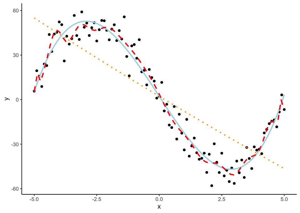
The red line is overfitted to the dataset and picks up too much of the unimportant pattern. The orange dotted line is underfit as it does not pick up enough of the pattern. The light blue, solid line is fit well to the dataset as it picks up the general pattern while not overfitting to the dataset.
To help with over-fitting, we could split the training data set again into a training and validation data set where the validation data set is what we “tune” our models on. The downside of this approach is that we will tend to start over-fitting the validation data set.
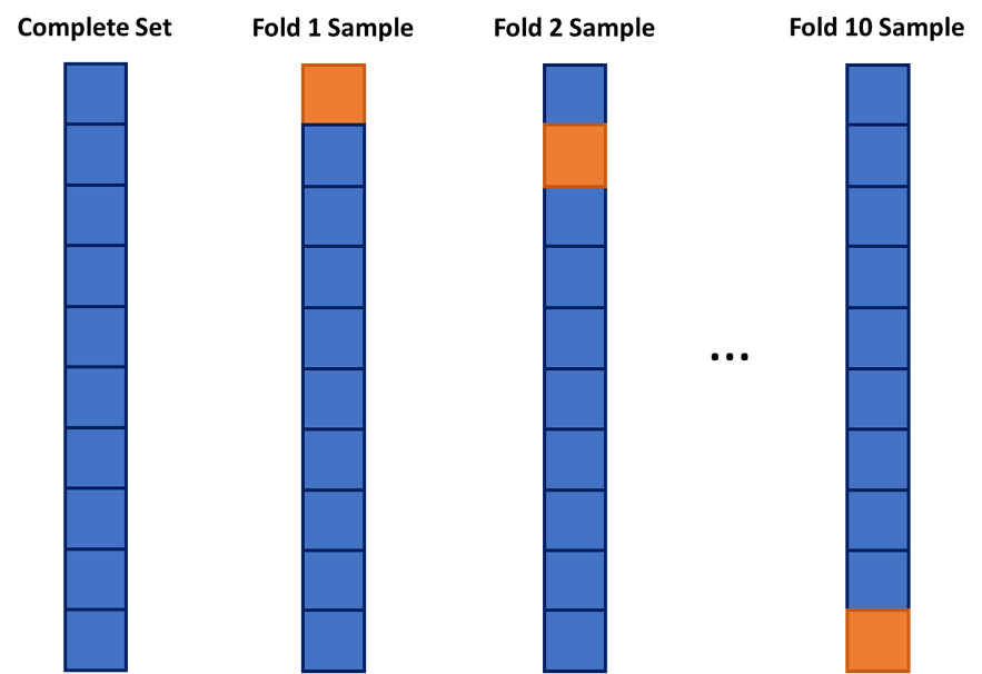
One approach to dealing with this is to use cross-validation. The idea of cross-validation is to divide your data set into k equally sized groups - called folds or samples. You leave one of the groups aside while building a model on the rest. You repeat this process of leaving one of the k folds out while building a model on the rest until each of the k folds has been left out once. We can evaluate a model by averaging the models’ effectiveness across all of the iterations. This process is highlighted below:
We will look at model building first without the use of cross-validation, but then with it.
Many different model metrics are used to help determine the validity of a model. Here of only SOME of the popular ones:
MAE (Mean Absolute Error) - the average of the absolute differences your predictions are from the truth.
MAPE (Mean Absolute Percentage Error) - the average of the absolute percentage differences your predictions are from the error.
MSE (Mean Squared Error) - the average of the squared differences your predictions are from the truth; also, the estimate of the variance of your errors from your model.
RMSE (Root Mean Squared Error) - the square root of the MSE; also, the standard deviation of your errors from your model.
In all of the above metrics, lower values represent a model that more highly predicts the target variable. However, these metrics might not always agree on which of the models is the best model.
Three of the above metrics are dependent on scale. Those metrics are the MAE, MSE, and RMSE:
Mean Absolute Error (MAE):
\[ MAE = \frac{1}{n} \sum_{i=1}^n |y_i - \hat{y}_i| \]
Mean Squared Error (MSE):
\[ MSE = \frac{1}{n} \sum_{i=1}^n (y_i - \hat{y}_i)^2 \]
Root Mean Squared Error (RMSE):
\[ RMSE = \sqrt(\frac{1}{n} \sum_{i=1}^n (y_i - \hat{y}_i)^2) \]
These metrics above are both scale dependent and symmetric. Scale dependent metrics are metrics that can only be compared to data with similar values for the data points. For example, we cannot compare a model trying to predict the price of a car with another model trying to predict the GDP of a country with MAE. An average error of $100,000 might be good for a model predicting GDP, but not as good for a model predicting price of a car. A symmetric metric is a metric that has the same meaning if the prediction is above the actual value as below the actual value. Again, for example, an error of $10,000 above a prediction is the same as an error $10,000 below a prediction.
The MAPE metric does not depend on scale, however, it is also not a symmetric metric.
Mean Absolute Percentage Error (MAPE):
\[ MAPE = \frac{1}{n} \sum_{i=1}^n |\frac{y_i - \hat{y}_i}{y_i}| \]
This final metric is both scale independent and asymmetric. Scale independent metrics are metrics that can be compared to data with any values for the data points. For example, we can compare a model trying to predict the price of a car with another model trying to predict the GDP of a country with MAPE. An average percentage error of 4% would be a worse model in context compared to a model with an average percentage error of 2.5%. An asymmetric metric is a metric that has a different meaning if the prediction is above the actual value as below the actual value. For example, a 5% error above is not the same as a 5% error below.
Which variables should you drop from your model? This is a common question for all modeling, but especially linear regression. In this section we will cover a popular variable selection technique - stepwise regression. This isn’t the only possible technique, but will be the primary focus here.
Stepwise regression techniques involve the three common methods:
Forward Selection
Backward Selection
Stepwise Selection
These techniques add or remove (depending on the technique) one variable at a time from your regression model to try and “improve” the model. There are a variety of different selection criteria to use to add or remove variables from a linear regression.
Let’s work through the process of forward selection. In forward selection, the initial model is empty (contains no variables, only the intercept). Each variable is then tried to see if it adds value based on a model metric. The variable that adds the most value is then added to the model. Then the remaining variables are again tested and the next most impactful variable is added to the model. This process repeats until either no more variables are available or no other variables improve the model metric.
Take a look at the picture below:
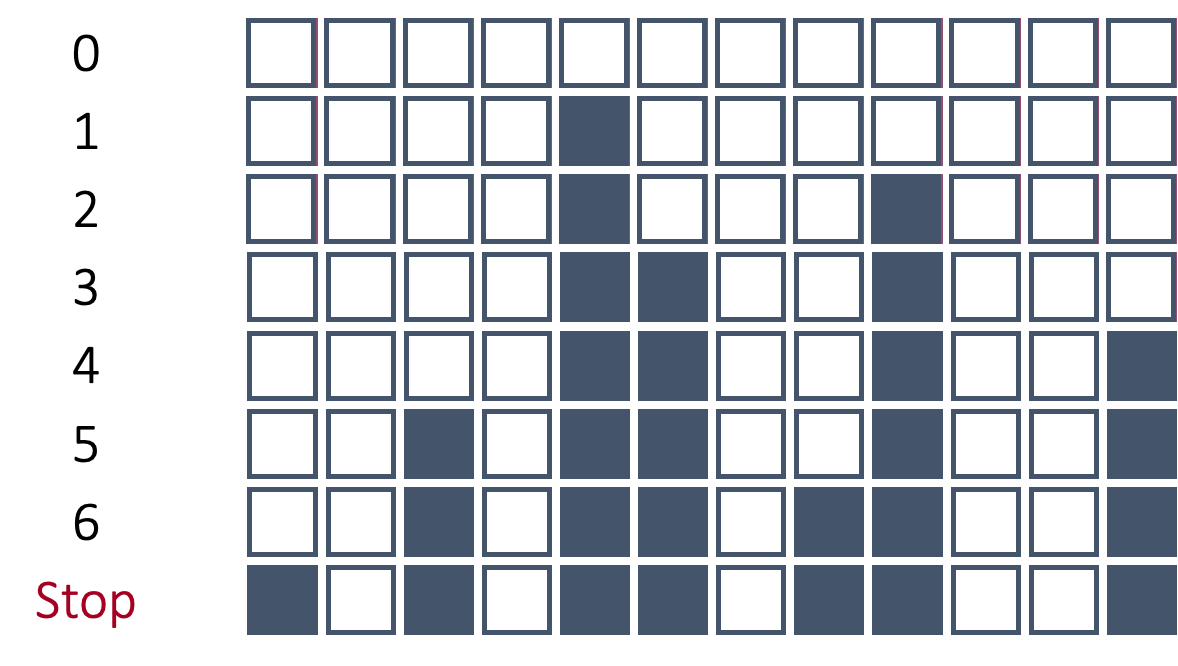
In the above example, after all of the variables were tested in models by themselves with the target, the 5th variable was deemed the best by the model metric. That variable is now in the model from this point forward. Next, all two variable models were built with every other variable added one at a time with the fifth variable. The combination of the 5th and 9th variables was deemed as the best combination from these options. Those two variables are now in the model going forward. This process stopped when no more variables improved the model metric on the overall model.
Forward selection is the least used technique because stepwise selection does the same as forward selection with an added benefit as discussed below.
In backward selection, the initial model is full (contains all variables, including the intercept). Each variable is then tried to see if it is worth keeping based on a specific model metric. The least worthy variable (or the one that hinders the model the most) is then dropped from the model. Then the remaining variables are again tested and the next least important variable is dropped from the model.
Take a look at the picture below:
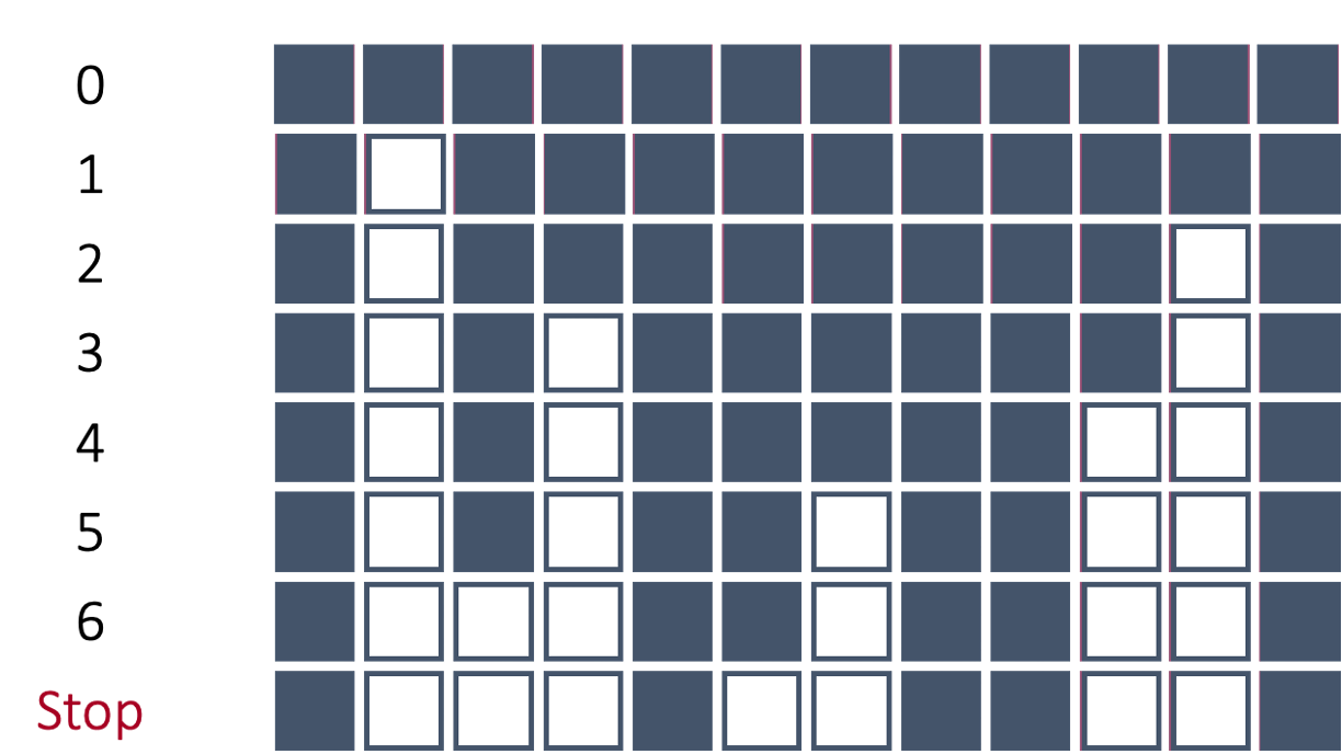
In the above example, the 2nd variable was deemed as the worst variable because the model improved the most (based on a model metric) with its deletion. Therefore, the 2nd variable is dropped from the model and cannot come back into the model. Next, each variable is again evaluated to see how the model improves with that variable’s deletion. The 11th variable is now deemed the worst and dropped. This process repeats until the model no longer improves with the deletion of another variable.
Backward selection is one of the most popular approaches to automatic model selection.
In stepwise selection, the initial model is empty (contains no variables, only the intercept) similar to forward selection. Each variable is then added one at a time to evaluate all single variable models to see which variable improves the model the most. The most important variable based on our model metric is then added to the model. Up until this point, it has been the same as forward selection. Next, all variables in the model (here only one) are tested to see if they are still helpful to the model by dropping all of them one at a time. This is similar to a backward selection at only this step. If they are hindering the model, they are dropped. Then the remaining variables are again tested and the next most impactful variable is added to the model. This process repeats until either no more variables are improving the model metric by adding or deleting variables.
Take a look at the picture below:
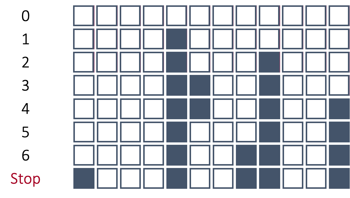
In the above picture the process starts off very similar to forward selection until we get to step 5. In step 5, the 6th variable is dropped from the model. In forward selection, if the 6th variable was added it could not be dropped. However, here that variable was evaluated to see if it still helped the model metric by being in the model. Since the model metric improved with the deletion of that variable, the variable was dropped.
All of the above techniques can be built with and without cross-validation. Both approaches are discussed in the following sections.
We will start without the use of cross-validation and only focusing on backward selection.
Let’s see how this works in each software!
Python has a built in recursive feature elimination (RFE) function inside of sklearn.feature_selection. However, there are some concerns with using that function. The biggest concern is the RFE function chooses variables in a linear regression based on the magnitude of the coefficients. This poses big problems in a linear regression model as we will see below.
First, let’s build a linear regression with the LinearRegression function from sklearn.linear_model and do backward selection with RFE. We put the LinearRegression object into the estimator option of the RFE function. Next, we need to figure out how many features we want to select. In the n_features_to_select option we can put any integer or the value of None. The None value will just select the “best” half of the variables from the model. From there we put our X_reduced and y objects in the fit function. Lastly, we get the variables from the RFE object with the support_ function and tie that to the respective variables using the columns function.
from sklearn.feature_selection import RFE
from sklearn.linear_model import LinearRegression
import pandas as pd

# Initialize model
model = LinearRegression()

# Set up Recursive Feature Elimination (RFE) to select top features
rfe = RFE(estimator = model, n_features_to_select = None)
rfe = rfe.fit(X_reduced, y)

# Get selected features
selected_features = X_reduced.columns[rfe.support_]

print("Selected features:", list(selected_features))
Selected features: ['OverallQual', 'GarageCars', 'ExterQual_TA', 'FullBath', 'TotRmsAbvGrd', 'KitchenQual_TA', 'Foundation_PConc', 'FireplaceQu_Missing', 'Fireplaces', 'BsmtQual_TA', 'ExterQual_Gd', 'Foundation_CBlock', 'FireplaceQu_Gd', 'KitchenQual_Gd', 'HalfBath', 'GarageCond_TA', 'HouseStyle_2Story', 'GarageQual_TA', 'GarageType_Missing', 'GarageCond_Missing', 'GarageYrBlt_was_missing', 'BsmtQual_Gd', 'KitchenQual_Fa', 'BsmtQual_Missing', 'LotConfig_CulDSac', 'FireplaceQu_TA', 'LotShape_IR2', 'GarageQual_Fa', 'GarageCond_Fa', 'BsmtQual_Fa', 'BldgType_Duplex', 'ExterQual_Fa', 'Condition1_Norm', 'BldgType_Twnhs', 'BldgType_2fmCon']That is a long list of variables printed out above. Remember, this is only half of the variables because we specified the n_features_to_select = None option. Instead, let’s pick out the top 10 variables by changing that option.
# Initialize model
model = LinearRegression()

# Set up Recursive Feature Elimination (RFE) to select top features
rfe = RFE(estimator = model, n_features_to_select = 10)
rfe = rfe.fit(X_reduced, y)

# Get selected features
selected_features = X_reduced.columns[rfe.support_]

print("Selected features:", list(selected_features))
Selected features: ['GarageCars', 'KitchenQual_TA', 'BsmtQual_TA', 'KitchenQual_Gd', 'BsmtQual_Gd', 'KitchenQual_Fa', 'BsmtQual_Missing', 'LotShape_IR2', 'BsmtQual_Fa', 'BldgType_Twnhs']Now that we a much more easily digestible list of the top 10 variables. One of the pitfalls of using the RFE function is that it doesn’t provide any notion of a cut-off based metric where all variables meeting a certain threshold are kept while others are eliminated. The choice of how many variables is completely up to the user.
Let’s examine what would happen if we change the scale of one of our variables. The OverallQual variable is on a scale of 1 to 10. Let’s change that scale to 0 to 1 by dividing that variable by 10. This doesn’t change any notion of the strength of the relationship between this variable at the target variable since we are just changing the scale. Let’s build a linear regression with this new dataset called X_new with our changed variable.
X_new = X_reduced.copy()

X_new['OverallQual'] = X_new['OverallQual']/10

model_new = sm.OLS(y, X_new).fit()

print(model_new.summary())
OLS Regression Results
==============================================================================
Dep. Variable: SalePrice R-squared: 0.829
Model: OLS Adj. R-squared: 0.818
Method: Least Squares F-statistic: 75.26
Date: Sat, 15 Nov 2025 Prob (F-statistic): 0.00
Time: 10:50:48 Log-Likelihood: -12977.
No. Observations: 1095 AIC: 2.609e+04
Df Residuals: 1028 BIC: 2.642e+04
Df Model: 66
Covariance Type: nonrobust
===========================================================================================
coef std err t P>|t| [0.025 0.975]
-------------------------------------------------------------------------------------------
const -8.745e+04 2.54e+05 -0.344 0.731 -5.86e+05 4.11e+05
OverallQual 1.243e+05 1.53e+04 8.126 0.000 9.43e+04 1.54e+05
GrLivArea 1.0898 23.844 0.046 0.964 -45.699 47.879
GarageCars 1.339e+04 3624.893 3.694 0.000 6276.531 2.05e+04
GarageArea 25.8692 11.854 2.182 0.029 2.609 49.129
TotalBsmtSF 13.2116 6.415 2.059 0.040 0.623 25.800
1stFlrSF 37.1809 24.551 1.514 0.130 -10.994 85.356
ExterQual_TA -1.643e+04 8375.482 -1.961 0.050 -3.29e+04 9.692
FullBath 2177.6897 3377.463 0.645 0.519 -4449.820 8805.199
TotRmsAbvGrd 2150.1420 1458.739 1.474 0.141 -712.304 5012.588
KitchenQual_TA -3.76e+04 6384.526 -5.890 0.000 -5.01e+04 -2.51e+04
YearBuilt 183.5406 99.159 1.851 0.064 -11.036 378.117
YearRemodAdd 136.7789 83.252 1.643 0.101 -26.585 300.143
Foundation_PConc 1.391e+04 5578.347 2.494 0.013 2968.437 2.49e+04
FireplaceQu_Missing 2719.7438 7145.154 0.381 0.704 -1.13e+04 1.67e+04
Fireplaces 1.127e+04 4350.193 2.592 0.010 2738.713 1.98e+04
GarageYrBlt -261.6592 92.929 -2.816 0.005 -444.012 -79.306
BsmtQual_TA -3.679e+04 6601.991 -5.573 0.000 -4.97e+04 -2.38e+04
ExterQual_Gd -1.173e+04 7482.799 -1.568 0.117 -2.64e+04 2953.250
GarageType_Detchd 9558.9692 9097.893 1.051 0.294 -8293.592 2.74e+04
Foundation_CBlock 1.342e+04 4979.062 2.695 0.007 3648.407 2.32e+04
GarageType_Attchd 1.226e+04 8993.147 1.363 0.173 -5387.657 2.99e+04
FireplaceQu_Gd -7087.3241 5448.909 -1.301 0.194 -1.78e+04 3604.929
LotFrontage -35.6152 62.515 -0.570 0.569 -158.287 87.056
OpenPorchSF -17.6777 17.953 -0.985 0.325 -52.906 17.551
2ndFlrSF 53.1360 24.650 2.156 0.031 4.765 101.507
HeatingQC_TA -6243.5810 3274.991 -1.906 0.057 -1.27e+04 182.849
KitchenQual_Gd -3.022e+04 5638.921 -5.360 0.000 -4.13e+04 -1.92e+04
WoodDeckSF 33.4070 9.319 3.585 0.000 15.120 51.694
HalfBath 919.7145 3260.459 0.282 0.778 -5478.201 7317.630
LotShape_Reg -3858.9488 2546.583 -1.515 0.130 -8856.043 1138.145
LotArea 0.1977 0.142 1.395 0.163 -0.080 0.476
GarageCond_TA 1.133e+04 1.11e+04 1.021 0.307 -1.04e+04 3.31e+04
HouseStyle_2Story -1.476e+04 4711.293 -3.133 0.002 -2.4e+04 -5516.886
CentralAir_Y 2660.7298 5988.337 0.444 0.657 -9090.031 1.44e+04
GarageType_BuiltIn 1.077e+04 1.04e+04 1.033 0.302 -9691.479 3.12e+04
GarageQual_TA -1.946e+04 1.05e+04 -1.853 0.064 -4.01e+04 1151.166
PavedDrive_Y 3224.5206 5564.756 0.579 0.562 -7695.056 1.41e+04
GarageType_Missing 8484.6693 3962.121 2.141 0.032 709.900 1.63e+04
GarageCond_Missing 8484.6693 3962.121 2.141 0.032 709.900 1.63e+04
GarageQual_Missing 8484.6693 3962.121 2.141 0.032 709.900 1.63e+04
GarageYrBlt_was_missing 8484.6693 3962.121 2.141 0.032 709.900 1.63e+04
BsmtQual_Gd -3.593e+04 5316.082 -6.758 0.000 -4.64e+04 -2.55e+04
BedroomAbvGr -1692.3586 2087.286 -0.811 0.418 -5788.186 2403.468
KitchenQual_Fa -3.751e+04 9832.196 -3.815 0.000 -5.68e+04 -1.82e+04
BsmtQual_Missing -2.512e+04 1.66e+04 -1.513 0.131 -5.77e+04 7458.243
LotConfig_CulDSac 1.241e+04 5473.956 2.266 0.024 1664.626 2.31e+04
FireplaceQu_TA -5272.0765 5524.834 -0.954 0.340 -1.61e+04 5569.164
HeatingQC_Gd -4929.1065 3348.159 -1.472 0.141 -1.15e+04 1640.900
LotShape_IR2 1.384e+04 6924.985 1.998 0.046 249.567 2.74e+04
GarageQual_Fa -2.549e+04 1.2e+04 -2.123 0.034 -4.9e+04 -1933.388
GarageCond_Fa 1.142e+04 1.3e+04 0.875 0.382 -1.42e+04 3.7e+04
BsmtQual_Fa -4.171e+04 9989.190 -4.176 0.000 -6.13e+04 -2.21e+04
Foundation_Slab 2737.4065 1.71e+04 0.160 0.873 -3.07e+04 3.62e+04
ScreenPorch 56.4523 19.636 2.875 0.004 17.921 94.983
EnclosedPorch 4.4598 19.374 0.230 0.818 -33.557 42.476
BldgType_Duplex -2.193e+04 7500.892 -2.924 0.004 -3.66e+04 -7212.060
LandContour_HLS 6639.3386 6447.555 1.030 0.303 -6012.533 1.93e+04
HeatingQC_Fa -2907.5365 7307.787 -0.398 0.691 -1.72e+04 1.14e+04
Condition1_Feedr -987.5563 6084.564 -0.162 0.871 -1.29e+04 1.1e+04
ExterQual_Fa -2.059e+04 1.46e+04 -1.411 0.159 -4.92e+04 8049.064
Condition1_Norm 1.247e+04 4066.459 3.068 0.002 4495.034 2.05e+04
PoolArea -76.3474 32.180 -2.373 0.018 -139.493 -13.202
BldgType_Twnhs -1.906e+04 7258.792 -2.626 0.009 -3.33e+04 -4820.314
HouseStyle_1.5Unf 5347.2965 1.04e+04 0.513 0.608 -1.51e+04 2.58e+04
HouseStyle_SFoyer 3841.6662 8117.844 0.473 0.636 -1.21e+04 1.98e+04
BldgType_2fmCon -1.267e+04 8102.544 -1.564 0.118 -2.86e+04 3230.109
LotConfig_Inside -600.4065 2769.771 -0.217 0.828 -6035.456 4834.643
PavedDrive_P 1252.2416 9240.160 0.136 0.892 -1.69e+04 1.94e+04
GarageType_CarPort 5815.4725 1.54e+04 0.378 0.705 -2.43e+04 3.6e+04
==============================================================================
Omnibus: 431.767 Durbin-Watson: 2.057
Prob(Omnibus): 0.000 Jarque-Bera (JB): 50780.630
Skew: -0.779 Prob(JB): 0.00
Kurtosis: 36.325 Cond. No. 1.28e+16
==============================================================================
Notes:
[1] Standard Errors assume that the covariance matrix of the errors is correctly specified.
[2] The smallest eigenvalue is 1.4e-21. This might indicate that there are
strong multicollinearity problems or that the design matrix is singular.The model’s ability to predict the target variable has not changed at all. The \(R^2\) value, adjusted \(R^2\) value, Log-Likelihood value, and F-statistic are all the exact same. This should not be surprising as the variable really isn’t any different except for the scale change. However, let’s examine the coefficient on that OverallQual variable. Notice how that variable coefficient is now 10 times larger than it was in our original linear regression model from the previous section. The standard error is now 10 times bigger as well. However, since we divide those two to get the test statistic (t column), the test statistic is the exact same between this new regression and the original one. That means that the p-value on that variable between the two models is also the exact same.
So it appears that nothing has really changed! However, let’s run the RFE function again.
# Initialize model
model = LinearRegression()

# Set up Recursive Feature Elimination (RFE) to select top features
rfe = RFE(estimator = model, n_features_to_select = 10)
rfe = rfe.fit(X_new, y)

# Get selected features
selected_features = X_new.columns[rfe.support_]

print("Selected features:", list(selected_features))
Selected features: ['OverallQual', 'KitchenQual_TA', 'BsmtQual_TA', 'KitchenQual_Gd', 'BsmtQual_Gd', 'KitchenQual_Fa', 'BsmtQual_Missing', 'LotShape_IR2', 'BsmtQual_Fa', 'BldgType_Twnhs']Notice how the OverallQual variable has now appeared in our top 10 list. But wait! I thought we just said that the model is no different and the variable has no different significance because the p-value did not change? Correct, but the coefficient did change because we changed the scale of the data. A variable’s coefficient in a linear regression is scale dependent because it is related to the interpretability of the variable. By changing the scale, we changed the interpretation, and unfortunately, the rankings of variables produced by the RFE function.
For this reason, I do not recommend using the RFE function for variable selection. One possible work around for this would be to scale the variables first. An example of that is shown below by building a pipeline (using the make_pipeline) function to standardize the variables first (StandardScaler) and then put them into the RFE function.
from sklearn.preprocessing import StandardScaler
from sklearn.feature_selection import RFE
from sklearn.linear_model import LinearRegression
from sklearn.pipeline import make_pipeline

# RFE with standardized features
model = LinearRegression()
pipeline = make_pipeline(StandardScaler(), RFE(model, n_features_to_select = 10))
pipeline.fit(X_reduced, y)
Pipeline(steps=[('standardscaler', StandardScaler()),
('rfe',
RFE(estimator=LinearRegression(), n_features_to_select=10))])In a Jupyter environment, please rerun this cell to show the HTML representation or trust the notebook. | steps | [('standardscaler', ...), ('rfe', ...)] | |
| transform_input | None | |
| memory | None | |
| verbose | False |
| copy | True | |
| with_mean | True | |
| with_std | True |
| estimator | LinearRegression() | |
| n_features_to_select | 10 | |
| step | 1 | |
| verbose | 0 | |
| importance_getter | 'auto' |
LinearRegression()
| fit_intercept | True | |
| copy_X | True | |
| tol | 1e-06 | |
| n_jobs | None | |
| positive | False |
# Access selected features from the RFE step
rfe_step = pipeline.named_steps['rfe']
selected_features = X_reduced.columns[rfe_step.support_]

print("Selected features:", list(selected_features))
Selected features: ['OverallQual', 'GarageCars', '1stFlrSF', 'KitchenQual_TA', 'Foundation_PConc', 'Foundation_CBlock', '2ndFlrSF', 'KitchenQual_Gd', 'BsmtQual_Gd', 'KitchenQual_Fa']Although better, this still doesn’t get around the problem of needing to select how many variables we want in the regression model. Also, since our variables are standardized, we have now lost some of the interpretability of the coefficients on the variables which is one of the biggest advantages to using linear regression. The coefficients are no longer telling what would happen with a single unit increase in a variable, but a single standard deviation increase in the variable. This makes interpretation for clients more challenging.
R has a built in step function that does recursive feature elimination such as backward selection. It uses likelihood based metrics to selection variables. We will use two of the most common ones: AIC and BIC (can also be referred to as SBC).
The AIC, or Akaike Information Criterion, was developed by statistician Hirotugu Akaike in the 1970’s and is defined by:
\[ AIC = n \log(\frac{SSE}{n}) + 2(p + 1) \]
In this case, the \(SSE\) is the sum of squared error from the model and \(2(p+1)\) is the “penalty”, where \(p\) is the number of variables in the model. A smaller AIC indicates a better model.
BIC, also known as the Bayesian Information Criterion (also called SBC or Schwarz Bayesian Information) was first developed by Gideon E. Schwarz, also back in the 1970’s and is defined by:
\[ BIC = n \log(\frac{SSE}{n}) + (p+1)\log (n) \]
In this case, “Likelihood” is the likelihood of the data and \((p+1)\log(n)\) is the “penalty”, where \(p\) is the number of variables in the model and \(n\) is the sample size. A smaller BIC indicates a better model.
To do backward elimination in R, you will use the step function. First, we need to define our full model (which is the model with all the predictor variables in it) similarly to how we did this above in our initial linear regression using the lm function. We must also define the lowest possible model (the intercept only model). To do this we can use the formula y ~ 1 to indicate that we want just the intercept term predicting the target variable. Inside of the step function we put our starting model, the full model, in first. For the scope of the model, you need to put the “smallest model” (using the lower option) to the “largest model” (using the upper option). The direction = "backward" option specifies that we want backward selection. The penalty (which indicates the criteria) can be controlled by defining the k option. A value of 2 will use the AIC criterion while a value of \(\log(n)\) will use the BIC criterion.
full_model <- lm(y ~ . , data = X_reduced)
empty_model <- lm(y ~ 1, data = X_reduced)

back_model <- step(full_model,
                  scope = list(lower = empty_model,
                               upper = full_model),
                  direction = "backward", k = 2, trace = FALSE)

summary(back_model)
Call:
lm(formula = y ~ OverallQual + GarageCars + GarageArea + TotalBsmtSF +
    FirstFlrSF + ExterQualTA + KitchenQualTA + YearBuilt + YearRemodAdd +
    FoundationPConc + Fireplaces + GarageYrBlt + BsmtQualTA +
    ExterQualGd + FoundationCBlock + FireplaceQuGd + SecondFlrSF +
    HeatingQCTA + KitchenQualGd + WoodDeckSF + LotShapeReg +
    LotArea + HouseStyle2Story + LotShapeIR1 + GarageQualTA +
    GarageTypeMissing + BsmtQualGd + KitchenQualFa + BsmtQualMissing +
    LotConfigCulDSac + FireplaceQuTA + LotShapeIR2 + GarageQualFa +
    BsmtQualFa + ScreenPorch + BldgTypeDuplex + ExterQualFa +
    Condition1Norm + PoolArea + BldgTypeTwnhs + BldgType2fmCon,
    data = X_reduced)

Residuals:
    Min      1Q  Median      3Q     Max
-346812  -14460     103   13912  269635

Coefficients:
                    Estimate Std. Error t value Pr(>|t|)
(Intercept)       -3.904e+05  2.173e+05  -1.797 0.072661 .
OverallQual        1.253e+04  1.470e+03   8.525  < 2e-16 ***
GarageCars         1.298e+04  3.456e+03   3.755 0.000183 ***
GarageArea         2.263e+01  1.113e+01   2.034 0.042176 *
TotalBsmtSF        1.678e+01  6.078e+00   2.761 0.005866 **
FirstFlrSF         4.159e+01  6.579e+00   6.322 3.80e-10 ***
ExterQualTA       -1.874e+04  8.106e+03  -2.312 0.020964 *
KitchenQualTA     -3.708e+04  6.157e+03  -6.022 2.38e-09 ***
YearBuilt          2.276e+02  8.369e+01   2.720 0.006644 **
YearRemodAdd       1.725e+02  7.861e+01   2.195 0.028413 *
FoundationPConc    1.234e+04  5.141e+03   2.400 0.016586 *
Fireplaces         1.077e+04  3.118e+03   3.454 0.000575 ***
GarageYrBlt       -2.211e+02  8.825e+01  -2.505 0.012393 *
BsmtQualTA        -3.433e+04  6.234e+03  -5.507 4.58e-08 ***
ExterQualGd       -1.387e+04  7.217e+03  -1.921 0.054942 .
FoundationCBlock   1.103e+04  4.461e+03   2.473 0.013554 *
FireplaceQuGd     -7.672e+03  4.064e+03  -1.888 0.059335 .
SecondFlrSF        5.904e+01  4.680e+00  12.616  < 2e-16 ***
HeatingQCTA       -4.091e+03  2.746e+03  -1.490 0.136549
KitchenQualGd     -2.992e+04  5.391e+03  -5.549 3.63e-08 ***
WoodDeckSF         3.526e+01  8.817e+00   3.999 6.81e-05 ***
LotShapeReg        8.672e+04  1.614e+04   5.374 9.49e-08 ***
LotArea            2.264e-01  1.350e-01   1.677 0.093820 .
HouseStyle2Story  -1.455e+04  4.337e+03  -3.356 0.000819 ***
LotShapeIR1        9.170e+04  1.614e+04   5.681 1.73e-08 ***
GarageQualTA      -1.335e+04  8.800e+03  -1.518 0.129432
GarageTypeMissing  1.644e+04  1.098e+04   1.498 0.134550
BsmtQualGd        -3.406e+04  5.108e+03  -6.668 4.19e-11 ***
KitchenQualFa     -3.950e+04  9.302e+03  -4.246 2.36e-05 ***
BsmtQualMissing   -1.910e+04  1.195e+04  -1.598 0.110277
LotConfigCulDSac   1.247e+04  4.777e+03   2.610 0.009182 **
FireplaceQuTA     -6.522e+03  4.286e+03  -1.522 0.128414
LotShapeIR2        1.042e+05  1.722e+04   6.052 1.99e-09 ***
GarageQualFa      -2.120e+04  1.047e+04  -2.025 0.043109 *
BsmtQualFa        -3.518e+04  9.640e+03  -3.649 0.000276 ***
ScreenPorch        5.242e+01  1.875e+01   2.795 0.005279 **
BldgTypeDuplex    -2.043e+04  6.659e+03  -3.067 0.002214 **
ExterQualFa       -2.461e+04  1.379e+04  -1.785 0.074483 .
Condition1Norm     1.179e+04  3.156e+03   3.734 0.000198 ***
PoolArea          -6.370e+01  3.036e+01  -2.098 0.036136 *
BldgTypeTwnhs     -1.726e+04  6.617e+03  -2.609 0.009206 **
BldgType2fmCon    -1.234e+04  7.683e+03  -1.607 0.108445
---
Signif. codes:  0 '***' 0.001 '**' 0.01 '*' 0.05 '.' 0.1 ' ' 1

Residual standard error: 34280 on 1053 degrees of freedom
Multiple R-squared:  0.8316,    Adjusted R-squared:  0.825
F-statistic: 126.8 on 41 and 1053 DF,  p-value: < 2.2e-16
From the list above we can see that the variables have been reduced down based on that AIC criterion. At each step the variable removed improved the model the most in that specific step by being the model that resulted in the lowest AIC value.
There are better options when it comes to doing forward, backward, and stepwise selection algorithms using cross-validation which is discussed in the next section.
Instead of looking at any of the stepwise regression techniques by using only the training data, from a machine learning standpoint, each step of the process is not evaluated on the training data, but on the cross-validation data sets. The model with the best average MSE (for example) in cross-validation is the one that moves on to the next step of the selection algorithm.
Let’s revisit the backward selection from above under this premise.

In first step of the backward selection process, we create models such that each model has exactly one predictor variable removed from it and calculate a model metric for each model. However, we do this across each cross-validation training set. For 10-fold cross-validation, that would be 10 separate first steps that create models removing only one variable. Next, we average the model metric across all training sets to see which is the worst variable. For example, the second variable is now the worst on average across all of the cross-validation datasets based on our model metric, not just the training set overall.
This same process is repeated across all of the steps until a final model is selected where removing any further variables does not improve the model based on the cross-validation model metrics.
Let’s see this in each software!
To gain the needed functionality for cross-validation recursive feature addition or subtraction, we need to use the mlxtend package on top of scikit-learn. Specifically, we will use the SequentialFeatureSelector function from mlxtend.feature_selection. Similar to before we will need to create our linear regression object with the LinearRegression function. This object will be an input to our SequentialFeatureSelector function called SFS from this point forward. In the k_features option we can put any integer value to set a certain number of features, the "best" option to pick the number of features that provides the best value of the model metric, or the "parsimonious" option to pick the number of features within one standard error of the true best model to try and make the model simpler. The forward = False option makes the function perform backward selection. The floating = False option means that once a variable is dropped it can no longer be added back to the model. The scoring option allows you to select your model metric. The options for a continuous target variable are the negative MSE, the negative RMSE, the negative MAE, and \(R^2\). The reason the first three are negative is that the function tries to maximize the optimization function. The cv option allows you to pick the number of cross-validation folds. Lastly, we just use the fit function with our predictor variables and target variable to fit the model. The variables are then printed below.
from mlxtend.feature_selection import SequentialFeatureSelector as SFS
from sklearn.linear_model import LinearRegression

lr = LinearRegression()

sfs = SFS(lr,
          k_features = "best",
          forward = False,
          floating = False,
          scoring = 'neg_mean_squared_error',
          cv = 10)

sfs = sfs.fit(X_reduced, y)

selected_features = list(sfs.k_feature_names_)
print("Selected features:", selected_features)
Selected features: ['const', 'OverallQual', 'GarageCars', '1stFlrSF', 'ExterQual_TA', 'KitchenQual_TA', 'YearBuilt', 'YearRemodAdd', 'Foundation_PConc', 'Fireplaces', 'GarageYrBlt', 'BsmtQual_TA', 'Foundation_CBlock', '2ndFlrSF', 'HeatingQC_TA', 'KitchenQual_Gd', 'WoodDeckSF', 'LotShape_Reg', 'HouseStyle_2Story', 'CentralAir_Y', 'GarageQual_TA', 'GarageType_Missing', 'GarageCond_Missing', 'GarageQual_Missing', 'GarageYrBlt_was_missing', 'BsmtQual_Gd', 'KitchenQual_Fa', 'BsmtQual_Missing', 'LotConfig_CulDSac', 'HeatingQC_Gd', 'LotShape_IR2', 'GarageQual_Fa', 'BsmtQual_Fa', 'ScreenPorch', 'BldgType_Duplex', 'ExterQual_Fa', 'Condition1_Norm', 'BldgType_Twnhs']Now we have variables determined by backward selection, but using cross-validation instead of just the whole training dataset.
To gain the needed functionality for cross-validation recursive feature addition or subtraction, we need to use the caret package. Specifically, we will use the train function from caret package along with the leaps package. The caret function can not handle our target variable and predictor variables being in separate objects. Therefore, we first use cbind to combine the target variable as a column to the predictor variables dataframe. Now we can use the new dataframe to put into caret with the typical formula structure we have used previously. The method = "leapBackward" option uses the leap package and its backward selection capabilities. You can think of caret as more of a wrapper function that puts a cross-validation spin on other functions. The tuneGrid option is where we specify what the model is tuning - here, the number of variables in the model. We are allowing that value to be anywhere from 1 variable all the way to 67 variables (the maximum amount we have). The metric option allows you to select your model metric. The options for a continuous target variable are the the RMSE, the MAE, and \(R^2\). The trControl = trainControl(method = 'cv', number = 10)) option allows you to pick the number of cross-validation folds. Lastly, we just look at the results element to view all of the possible model metrics across all tuning options and the bestTune element for it to tell us the optimal tuning value (optimal number of variables).
library(caret)
library(leaps)

set.seed(1234)

df <- cbind(y, X_reduced)

step_model <- caret::train(y ~ ., data = df,
                    method = "leapBackward",
                    tuneGrid = data.frame(nvmax = 1:67),
                    metric = "RMSE",
                    trControl = trainControl(method = 'cv',
                                             number = 10))
Reordering variables and trying again:Reordering variables and trying again:Reordering variables and trying again:Reordering variables and trying again:Reordering variables and trying again:Reordering variables and trying again:Reordering variables and trying again:Reordering variables and trying again:Reordering variables and trying again:Reordering variables and trying again:Reordering variables and trying again:step_model$results nvmax RMSE Rsquared MAE RMSESD RsquaredSD MAESD
1 1 49977.95 0.6379845 34413.62 8212.437 0.04056464 3444.893
2 2 45459.07 0.7041046 30790.61 7926.356 0.06412756 2460.768
3 3 42465.75 0.7458165 27781.02 10450.149 0.08616763 3338.279
4 4 41511.86 0.7594901 27182.04 10922.164 0.08467277 3508.469
5 5 41232.78 0.7619850 27029.26 10724.738 0.08285458 3368.540
6 6 40515.83 0.7702644 26542.27 11085.117 0.08570367 3569.525
7 7 40557.45 0.7698225 26624.11 11118.410 0.08590971 3648.460
8 8 40973.91 0.7663612 26311.93 12328.873 0.09694029 3473.413
9 9 40920.45 0.7673650 26132.34 12368.379 0.09692516 3281.338
10 10 40891.75 0.7691093 26121.63 12982.862 0.10313762 3490.216
11 11 40407.44 0.7740602 25719.59 13149.909 0.10591740 3511.174
12 12 40086.49 0.7772255 25407.08 13189.867 0.10694073 3469.621
13 13 39920.99 0.7784748 25189.05 12924.188 0.10432318 3373.224
14 14 40055.09 0.7780948 25130.63 13664.794 0.11034048 3555.922
15 15 40027.19 0.7777532 25160.91 13713.477 0.10972704 3604.560
16 16 39952.86 0.7789035 25093.18 13907.709 0.11048947 3634.715
17 17 40130.90 0.7767144 25084.03 14285.208 0.11509638 3603.802
18 18 40144.12 0.7765038 25034.20 14387.396 0.11566260 3630.875
19 19 39945.66 0.7787613 24872.55 14549.435 0.11747833 3831.055
20 20 40063.67 0.7767741 24996.00 14397.179 0.11519606 3922.747
21 21 39969.37 0.7780789 24931.91 14486.828 0.11591690 3728.593
22 22 39953.99 0.7779197 24971.49 14551.285 0.11614572 3767.608
23 23 39785.69 0.7796607 24909.19 14533.895 0.11584043 3765.717
24 24 39916.94 0.7784775 24981.24 14426.799 0.11540880 3685.338
25 25 39699.18 0.7806454 24851.48 14528.324 0.11682734 3854.198
26 26 39704.56 0.7807152 24870.64 14608.020 0.11726875 3959.261
27 27 40416.33 0.7725864 24987.20 15544.998 0.12506026 4233.939
28 28 40383.56 0.7731801 24822.57 15512.248 0.12390513 4100.529
29 29 40305.45 0.7737329 24731.46 15470.632 0.12363976 4354.071
30 30 40056.99 0.7764172 24485.28 15399.939 0.12305452 4372.851
31 31 39986.16 0.7769655 24473.29 15501.730 0.12407998 4427.617
32 32 39982.40 0.7772986 24533.92 15370.374 0.12225357 4428.186
33 33 40078.20 0.7762794 24540.73 15471.316 0.12317933 4392.251
34 34 40072.85 0.7762712 24504.77 15519.193 0.12370677 4364.689
35 35 39994.33 0.7771654 24476.86 15587.080 0.12408588 4376.086
36 36 39875.70 0.7784654 24400.96 15459.717 0.12333587 4240.014
37 37 39826.02 0.7791110 24300.89 15446.524 0.12314726 4076.386
38 38 39782.30 0.7797330 24265.98 15455.216 0.12338025 4015.840
39 39 39650.56 0.7810700 24113.85 15499.395 0.12376346 4076.217
40 40 39632.19 0.7816386 24084.26 15486.285 0.12379773 4083.176
41 41 39598.18 0.7822372 24153.47 15466.681 0.12352486 4041.807
42 42 39622.24 0.7815976 24081.13 15540.767 0.12454139 4045.688
43 43 39561.52 0.7821294 23985.83 15552.600 0.12450185 4121.165
44 44 39966.59 0.7795448 24069.00 16607.859 0.13294156 4201.958
45 45 39928.10 0.7807139 23893.63 16903.187 0.13441011 4157.105
46 46 39914.54 0.7808068 23879.04 16821.878 0.13352255 4051.365
47 47 39940.75 0.7803566 23891.62 16784.536 0.13312778 4087.454
48 48 39716.17 0.7826885 23752.77 16911.578 0.13449402 4172.458
49 49 39633.76 0.7827437 23719.88 16764.291 0.13355197 4233.713
50 50 39559.65 0.7829264 23687.68 16880.181 0.13451861 4260.193
51 51 39598.29 0.7831982 23580.80 17133.632 0.13420387 4371.630
52 52 39681.14 0.7823658 23627.00 17186.287 0.13467743 4350.324
53 53 39742.77 0.7817784 23568.37 17401.183 0.13590109 4352.411
54 54 39818.21 0.7811504 23607.73 17465.744 0.13610029 4347.436
55 55 39599.38 0.7831875 23472.50 17496.448 0.13695933 4232.871
56 56 39577.67 0.7834730 23472.62 17487.743 0.13680190 4245.662
57 57 39605.79 0.7831680 23458.07 17490.397 0.13686366 4229.525
58 58 39630.70 0.7829122 23475.12 17413.561 0.13659894 4140.855
59 59 39699.14 0.7819132 23530.27 17505.559 0.13788998 4242.893
60 60 39667.30 0.7821748 23536.38 17406.683 0.13715344 4223.407
61 61 39636.06 0.7826257 23517.75 17395.808 0.13718217 4197.986
62 62 39603.88 0.7830190 23490.82 17420.746 0.13742688 4209.628
63 63 39471.35 0.7840201 23392.04 17337.493 0.13645436 4246.797
64 64 39463.18 0.7838501 23358.98 17313.428 0.13671501 4225.027
65 65 39461.20 0.7838297 23353.78 17318.364 0.13675203 4203.101
66 66 39361.68 0.7848449 23251.27 17331.697 0.13704860 4138.985
67 67 39354.33 0.7847572 23283.06 17356.823 0.13720255 4218.298step_model$bestTune nvmax
67 67Now we have variables determined by backward selection, but using cross-validation instead of just the whole training dataset.
Let’s revisit the forward selection approach with cross-validation.
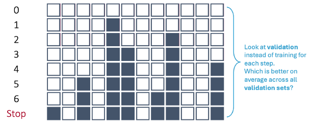
In first step of the forward selection process, we create models such that each model has exactly one predictor variable and calculate a model metric for each model. However, we do this across each cross-validation training set. For 10-fold cross-validation, that would be 10 separate first steps that create models with only one variable. Next, we average the model metric across all training sets to see which is the best variable. For example, the 5th variable is now the best on average across all of the cross-validation datasets based on our model metric, not just the training set overall.
This same process is repeated across all of the steps until a final model is selected where adding any further variables does not improve the model based on the cross-validation model metrics.
Let’s see this in each software!
To gain the needed functionality for cross-validation recursive feature addition or subtraction, we need to use the mlxtend package on top of scikit-learn. Specifically, we will use the SequentialFeatureSelector function from mlxtend.feature_selection. Similar to before we will need to create our linear regression object with the LinearRegression function. This object will be an input to our SFS function. In the k_features option we can put any integer value to set a certain number of features, the "best" option to pick the number of features that provides the best value of the model metric, or the "parsimonious" option to pick the number of features within one standard error of the true best model to try and make the model simpler. The forward = True option makes the function perform forward selection. The floating = False option means that once a variable is added it can no longer be dropped out of the model. The scoring option allows you to select your model metric. The options for a continuous target variable are the negative MSE, the negative RMSE, the negative MAE, and \(R^2\). The reason the first three are negative is that the function tries to maximize the optimization function. The cv option allows you to pick the number of cross-validation folds. Lastly, we just use the fit function with our predictor variables and target variable to fit the model. The variables are then printed below.
from mlxtend.feature_selection import SequentialFeatureSelector as SFS
from sklearn.linear_model import LinearRegression

lr = LinearRegression()

sfs = SFS(lr,
          k_features = "best",
          forward = True,
          floating = False,
          scoring = 'neg_mean_squared_error',
          cv = 10)

sfs = sfs.fit(X_reduced, y)

selected_features = list(sfs.k_feature_names_)
print("Selected features:", selected_features)
Selected features: ['const', 'OverallQual', 'GrLivArea', 'GarageCars', 'ExterQual_TA', 'KitchenQual_TA', 'YearBuilt', 'YearRemodAdd', 'Foundation_PConc', 'Fireplaces', 'GarageYrBlt', 'BsmtQual_TA', 'Foundation_CBlock', 'HeatingQC_TA', 'KitchenQual_Gd', 'WoodDeckSF', 'LotShape_Reg', 'HouseStyle_2Story', 'GarageQual_TA', 'GarageType_Missing', 'BsmtQual_Gd', 'KitchenQual_Fa', 'BsmtQual_Missing', 'LotConfig_CulDSac', 'HeatingQC_Gd', 'LotShape_IR2', 'GarageQual_Fa', 'BsmtQual_Fa', 'ScreenPorch', 'BldgType_Duplex', 'LandContour_HLS', 'ExterQual_Fa', 'Condition1_Norm', 'BldgType_Twnhs', 'BldgType_2fmCon']Now we have variables determined by forward selection, but using cross-validation instead of just the whole training dataset.
To gain the needed functionality for cross-validation recursive feature addition or subtraction, we need to use the caret package. Specifically, we will use the train function from caret package along with the leaps package. The caret function can not handle our target variable and predictor variables being in separate objects. Therefore, we first use cbind to combine the target variable as a column to the predictor variables dataframe. Now we can use the new dataframe to put into caret with the typical formula structure we have used previously. The method = "leapForward" option uses the leap package and its forward selection capabilities. You can think of caret as more of a wrapper function that puts a cross-validation spin on other functions. The tuneGrid option is where we specify what the model is tuning - here, the number of variables in the model. We are allowing that value to be anywhere from 1 variable all the way to 67 variables (the maximum amount we have). The metric option allows you to select your model metric. The options for a continuous target variable are the the RMSE, the MAE, and \(R^2\). The trControl = trainControl(method = 'cv', number = 10)) option allows you to pick the number of cross-validation folds. Lastly, we just look at the results element to view all of the possible model metrics across all tuning options and the bestTune element for it to tell us the optimal tuning value (optimal number of variables).
library(caret)
library(leaps)

set.seed(1234)

df <- cbind(y, X_reduced)

step_model <- caret::train(y ~ ., data = df,
                    method = "leapForward",
                    tuneGrid = data.frame(nvmax = 1:67),
                    metric = "RMSE",
                    trControl = trainControl(method = 'cv',
                                             number = 10))
Reordering variables and trying again:Reordering variables and trying again:Reordering variables and trying again:Reordering variables and trying again:Reordering variables and trying again:Reordering variables and trying again:Reordering variables and trying again:Reordering variables and trying again:Reordering variables and trying again:Reordering variables and trying again:Reordering variables and trying again:step_model$results nvmax RMSE Rsquared MAE RMSESD RsquaredSD MAESD
1 1 49977.95 0.6379845 34413.62 8212.437 0.04056464 3444.893
2 2 44065.22 0.7236820 29698.01 9080.063 0.06922790 3552.727
3 3 43959.81 0.7315774 28588.91 11952.421 0.09722373 3394.215
4 4 41405.17 0.7646045 26578.42 12641.364 0.10132140 3666.772
5 5 40930.80 0.7685289 26140.76 12428.316 0.09850066 3550.235
6 6 40580.10 0.7715237 25851.00 12428.278 0.09852391 3555.710
7 7 40614.83 0.7718889 25677.77 12844.802 0.10250808 3575.288
8 8 40770.84 0.7697826 25715.47 12993.562 0.10371694 3599.772
9 9 40771.36 0.7694843 25615.29 13060.696 0.10410918 3518.613
10 10 40807.45 0.7689106 25702.82 13091.477 0.10468397 3594.819
11 11 40623.32 0.7710256 25623.70 13097.755 0.10463381 3621.150
12 12 40635.14 0.7710461 25676.27 13134.346 0.10432781 3610.291
13 13 40561.27 0.7722723 25584.74 13324.333 0.10594470 3625.322
14 14 40098.83 0.7768163 25434.80 13515.728 0.10798838 3597.406
15 15 40184.54 0.7766575 25450.00 14008.865 0.11218369 3592.515
16 16 40025.08 0.7794208 25256.63 14931.740 0.11976550 3964.034
17 17 39780.53 0.7817577 25086.30 14912.751 0.11959949 4018.490
18 18 39679.96 0.7827848 24882.23 14869.034 0.12006461 3993.534
19 19 39657.32 0.7834076 24894.52 15307.443 0.12532356 4071.206
20 20 39572.19 0.7843185 24858.74 14982.236 0.12306155 3841.339
21 21 39573.42 0.7843582 24851.08 14928.639 0.12236263 3795.297
22 22 39397.90 0.7859510 24677.34 14522.204 0.11734907 3566.537
23 23 39367.46 0.7850693 24575.66 14240.205 0.11361569 3536.541
24 24 39414.66 0.7849372 24686.48 14175.075 0.11309018 3488.096
25 25 39474.40 0.7844007 24747.41 14161.640 0.11342905 3456.114
26 26 39578.96 0.7831461 24811.15 14074.448 0.11250030 3452.923
27 27 39655.35 0.7822218 24791.92 14091.837 0.11273754 3335.499
28 28 39315.78 0.7855275 24381.90 13939.011 0.11117948 3412.122
29 29 39169.89 0.7871236 24106.80 14003.690 0.11185007 3473.081
30 30 38918.10 0.7894983 24105.75 13891.763 0.11083610 3581.401
31 31 38822.17 0.7904751 23959.28 13951.145 0.11108685 3733.772
32 32 38794.17 0.7906649 23952.79 13903.261 0.11104066 3700.344
33 33 38754.62 0.7909585 23921.95 13950.831 0.11151265 3727.513
34 34 38710.70 0.7915131 23852.98 13913.792 0.11122430 3684.245
35 35 38724.13 0.7915973 23873.10 13911.358 0.11099673 3647.690
36 36 39132.66 0.7887345 23958.74 14968.882 0.11951394 3707.031
37 37 39780.57 0.7818177 24137.27 15642.427 0.12465807 3841.972
38 38 39817.20 0.7811496 24167.05 15621.243 0.12463474 3853.508
39 39 40001.31 0.7789784 24081.23 15714.562 0.12581521 3618.279
40 40 39992.88 0.7791316 24097.60 15728.788 0.12576006 3685.442
41 41 40164.43 0.7780223 24032.72 15845.784 0.12598815 3628.286
42 42 40021.34 0.7791569 23976.97 15765.739 0.12558955 3657.248
43 43 39971.67 0.7796162 24019.00 15778.099 0.12583691 3678.519
44 44 39862.00 0.7806290 23978.73 15772.700 0.12592640 3723.733
45 45 39877.22 0.7804828 23951.71 15834.151 0.12562599 3700.080
46 46 39711.25 0.7820456 23798.48 15948.036 0.12634593 3777.755
47 47 39747.55 0.7811853 23770.65 16114.052 0.12831183 3934.280
48 48 39749.02 0.7811050 23749.35 16179.819 0.12866672 4032.216
49 49 39748.42 0.7818975 23680.21 16473.427 0.12882695 4116.792
50 50 39534.79 0.7835799 23559.42 16482.941 0.12956359 3982.863
51 51 39532.76 0.7837670 23477.78 16765.908 0.13137223 4055.245
52 52 39546.02 0.7835880 23454.57 16933.757 0.13268014 4172.260
53 53 39394.10 0.7850185 23351.60 17051.009 0.13361689 4237.608
54 54 39355.82 0.7851866 23281.07 17050.263 0.13392387 4185.059
55 55 39394.05 0.7847251 23340.38 17081.916 0.13410549 4136.081
56 56 39432.46 0.7842432 23351.63 17093.708 0.13398623 4161.194
57 57 39379.60 0.7844638 23333.66 16939.348 0.13327685 4148.934
58 58 39318.33 0.7850504 23304.70 16895.765 0.13306264 4111.241
59 59 39482.48 0.7833044 23406.70 17002.214 0.13449369 4146.715
60 60 39465.09 0.7835235 23390.29 16953.619 0.13396022 4163.804
61 61 39398.47 0.7842722 23382.22 16914.154 0.13376750 4154.823
62 62 39400.28 0.7843006 23378.57 16912.181 0.13378026 4141.875
63 63 39306.84 0.7852101 23292.37 16924.075 0.13353777 4174.018
64 64 39289.21 0.7850404 23264.02 16920.491 0.13389910 4189.387
65 65 39304.51 0.7847474 23256.88 16903.714 0.13377204 4149.325
66 66 39215.43 0.7856952 23165.20 16933.618 0.13418146 4094.718
67 67 39183.10 0.7858519 23181.70 16962.298 0.13441327 4165.847step_model$bestTune nvmax
34 34Now we have variables determined by forward selection, but using cross-validation instead of just the whole training dataset.
Let’s revisit the stepwise selection approach with cross-validation.
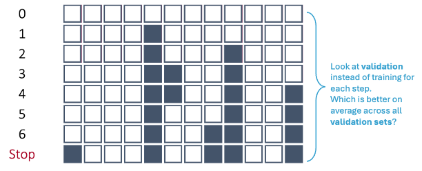
In first step of the stepwise selection process, we create models such that each model has exactly one predictor variable and calculate a model metric for each model. However, we do this across each cross-validation training set. For 10-fold cross-validation, that would be 10 separate first steps that create models with only one variable. Next, we average the model metric across all training sets to see which is the best variable. For example, the 5th variable is now the best on average across all of the cross-validation datasets based on our model metric, not just the training set overall.
This same process is repeated across all of the steps until a final model is selected where adding any further variables does not improve the model based on the cross-validation model metrics. Remember, the difference between forward and stepwise selection is that we are also evaluating each variable added to the model at each step to see if deleting that variable improves the model metric.
Let’s see this in each software!
To gain the needed functionality for cross-validation recursive feature addition or subtraction, we need to use the mlxtend package on top of scikit-learn. Specifically, we will use the SequentialFeatureSelector function from mlxtend.feature_selection. Similar to before we will need to create our linear regression object with the LinearRegression function. This object will be an input to our SFS function. In the k_features option we can put any integer value to set a certain number of features, the "best" option to pick the number of features that provides the best value of the model metric, or the "parsimonious" option to pick the number of features within one standard error of the true best model to try and make the model simpler. The forward = True option makes the function perform forward selection. The floating = True option means that once a variable is added it is evaluated at each step to be dropped out of the model - stepwise selection. The scoring option allows you to select your model metric. The options for a continuous target variable are the negative MSE, the negative RMSE, the negative MAE, and \(R^2\). The reason the first three are negative is that the function tries to maximize the optimization function. The cv option allows you to pick the number of cross-validation folds. Lastly, we just use the fit function with our predictor variables and target variable to fit the model. The variables are then printed below.
from mlxtend.feature_selection import SequentialFeatureSelector as SFS
from sklearn.linear_model import LinearRegression

lr = LinearRegression()

sfs = SFS(lr,
          k_features = "best",
          forward = True,
          floating = True,
          scoring = 'neg_mean_squared_error',
          cv = 10)

sfs = sfs.fit(X_reduced, y)

selected_features = list(sfs.k_feature_names_)
print("Selected features:", selected_features)
Selected features: ['const', 'OverallQual', 'GrLivArea', 'GarageCars', 'ExterQual_TA', 'KitchenQual_TA', 'YearBuilt', 'YearRemodAdd', 'Foundation_PConc', 'Fireplaces', 'GarageYrBlt', 'BsmtQual_TA', 'Foundation_CBlock', 'HeatingQC_TA', 'KitchenQual_Gd', 'WoodDeckSF', 'LotShape_Reg', 'HouseStyle_2Story', 'GarageQual_TA', 'GarageType_Missing', 'BsmtQual_Gd', 'KitchenQual_Fa', 'BsmtQual_Missing', 'LotConfig_CulDSac', 'HeatingQC_Gd', 'LotShape_IR2', 'GarageQual_Fa', 'BsmtQual_Fa', 'ScreenPorch', 'BldgType_Duplex', 'LandContour_HLS', 'ExterQual_Fa', 'Condition1_Norm', 'BldgType_Twnhs', 'BldgType_2fmCon']Now we have variables determined by forward selection, but using cross-validation instead of just the whole training dataset.
To gain the needed functionality for cross-validation recursive feature addition or subtraction, we need to use the caret package. Specifically, we will use the train function from caret package along with the leaps package. The caret function can not handle our target variable and predictor variables being in separate objects. Therefore, we first use cbind to combine the target variable as a column to the predictor variables dataframe. Now we can use the new dataframe to put into caret with the typical formula structure we have used previously. The method = "leapSeq" option uses the leap package and its stepwise selection capabilities. You can think of caret as more of a wrapper function that puts a cross-validation spin on other functions. The tuneGrid option is where we specify what the model is tuning - here, the number of variables in the model. We are allowing that value to be anywhere from 1 variable all the way to 67 variables (the maximum amount we have). The metric option allows you to select your model metric. The options for a continuous target variable are the the RMSE, the MAE, and \(R^2\). The trControl = trainControl(method = 'cv', number = 10)) option allows you to pick the number of cross-validation folds. Lastly, we just look at the results element to view all of the possible model metrics across all tuning options and the bestTune element for it to tell us the optimal tuning value (optimal number of variables).
library(caret)
library(leaps)

set.seed(1234)

df <- cbind(y, X_reduced)

step_model <- caret::train(y ~ ., data = df,
                    method = "leapSeq",
                    tuneGrid = data.frame(nvmax = 1:67),
                    metric = "RMSE",
                    trControl = trainControl(method = 'cv',
                                             number = 10))
Reordering variables and trying again:Reordering variables and trying again:Reordering variables and trying again:Reordering variables and trying again:Reordering variables and trying again:Reordering variables and trying again:Reordering variables and trying again:Reordering variables and trying again:Reordering variables and trying again:Reordering variables and trying again:Reordering variables and trying again:step_model$results nvmax RMSE Rsquared MAE RMSESD RsquaredSD MAESD
1 1 49977.95 0.6379845 34413.62 8212.437 0.04056464 3444.893
2 2 44065.22 0.7236820 29698.01 9080.063 0.06922790 3552.727
3 3 43959.81 0.7315774 28588.91 11952.421 0.09722373 3394.215
4 4 41385.80 0.7651593 26646.54 12589.854 0.10071069 3678.962
5 5 40915.00 0.7688240 26163.41 12441.946 0.09865031 3536.018
6 6 40676.68 0.7706442 25765.46 13091.796 0.10906020 3366.123
7 7 41001.51 0.7689376 25920.62 13203.642 0.10657099 3580.137
8 8 41683.48 0.7586253 26274.89 13310.408 0.10841429 3967.855
9 9 41410.45 0.7631968 26423.08 13241.886 0.10385529 4105.901
10 10 41346.10 0.7636332 26148.96 13245.831 0.10455033 3549.424
11 11 41066.23 0.7656376 26149.75 13039.837 0.10261311 3809.183
12 12 41012.85 0.7681520 26158.04 13399.593 0.10475922 3819.745
13 13 40714.48 0.7708829 25755.85 13357.779 0.10561859 3895.819
14 14 39976.27 0.7788409 25273.08 13919.716 0.11245519 3859.413
15 15 40632.19 0.7735642 25279.67 14784.517 0.12111108 3608.832
16 16 40024.92 0.7791530 25156.13 13893.394 0.11247398 3716.092
17 17 40371.06 0.7766387 25126.92 14862.003 0.12242422 3653.285
18 18 39671.80 0.7845788 24852.23 13882.874 0.11071291 3145.013
19 19 39589.66 0.7846719 24937.04 14834.571 0.12255120 3722.400
20 20 40167.10 0.7771359 25051.46 15796.790 0.13011108 3979.132
21 21 39928.82 0.7796240 24914.30 15558.199 0.12877594 3528.895
22 22 39185.37 0.7869539 24601.73 14026.018 0.11263143 3297.538
23 23 39122.74 0.7877369 24403.19 14186.862 0.11348909 3437.689
24 24 39151.99 0.7873541 24556.36 14268.504 0.11413450 3483.806
25 25 40093.76 0.7785300 24725.96 15583.595 0.12868603 3788.524
26 26 40445.87 0.7734753 24797.52 16900.725 0.13900480 4392.804
27 27 39409.33 0.7834902 24077.82 14722.036 0.11769956 3666.450
28 28 39361.69 0.7841777 24063.53 14890.935 0.11871143 4257.916
29 29 39569.96 0.7810188 24046.21 14879.856 0.11739244 4164.832
30 30 39392.82 0.7834821 24057.65 15344.031 0.12396216 4210.025
31 31 39439.54 0.7833485 24202.73 15369.984 0.12356606 4477.332
32 32 39108.98 0.7855831 23836.60 15462.525 0.12448234 4202.464
33 33 38958.62 0.7888182 24155.80 14367.672 0.11557569 3958.726
34 34 39488.56 0.7848993 24129.74 15697.443 0.12548076 4076.687
35 35 39557.17 0.7839702 24161.43 15586.259 0.12480791 4062.423
36 36 39955.07 0.7788572 24044.28 16353.918 0.13149733 4014.116
37 37 39846.83 0.7806146 23985.92 16188.965 0.12964170 4139.640
38 38 39938.62 0.7797187 23926.24 16579.452 0.13382757 4242.013
39 39 39880.19 0.7805330 23735.36 16507.821 0.13223658 4026.990
40 40 39814.72 0.7807159 23936.26 15879.872 0.12678443 3966.677
41 41 40077.64 0.7797481 23920.19 16390.405 0.13040420 3803.286
42 42 39699.85 0.7818969 23798.73 15962.242 0.12754635 3948.006
43 43 39453.96 0.7835274 23548.57 16064.483 0.12866461 4025.484
44 44 39750.26 0.7808150 23736.51 16622.800 0.13203358 4047.917
45 45 39518.41 0.7841275 23580.52 17003.245 0.13665755 4250.253
46 46 39204.59 0.7857076 23596.76 16034.220 0.12957400 4102.616
47 47 39711.45 0.7829903 23672.14 17027.656 0.13308371 4257.897
48 48 39264.24 0.7867628 23450.99 17058.911 0.13257106 4135.151
49 49 39300.07 0.7859552 23448.80 16647.144 0.13053610 4283.283
50 50 39615.70 0.7837961 23410.55 17315.888 0.13513964 4339.327
51 51 39681.43 0.7830901 23259.00 18116.789 0.14171337 4667.237
52 52 39025.81 0.7885568 22996.61 17298.791 0.13607982 4413.565
53 53 39485.99 0.7854001 23300.71 18248.854 0.14317908 4540.477
54 54 39504.89 0.7843308 23428.94 17501.740 0.13707069 4159.021
55 55 39090.43 0.7898445 23137.79 17425.162 0.13573422 4122.184
56 56 38964.96 0.7907073 23085.90 17413.057 0.13537223 4276.133
57 57 39198.28 0.7875097 23113.53 17712.275 0.13899406 4238.036
58 58 39482.53 0.7836705 23329.77 17893.495 0.14060029 4511.961
59 59 39288.98 0.7862310 23413.65 17208.625 0.13447600 4182.626
60 60 39706.02 0.7818555 23564.06 17849.330 0.14125174 4294.174
61 61 39485.19 0.7832632 23394.60 17480.585 0.13715249 4391.239
62 62 39578.39 0.7834418 23408.55 17845.273 0.14153842 4200.179
63 63 38868.21 0.7902382 23082.09 17480.250 0.13799571 4428.751
64 64 38912.54 0.7904563 23041.81 17228.654 0.13575531 4163.532
65 65 38935.47 0.7889639 23097.37 16981.691 0.13462921 4297.540
66 66 39182.27 0.7869607 23098.31 17239.410 0.13564852 4252.665
67 67 39354.33 0.7847572 23283.06 17356.823 0.13720255 4218.298step_model$bestTune nvmax
63 63Now we have variables determined by stepwise selection, but using cross-validation instead of just the whole training dataset.
There are some cautions that come with automatic selection techniques.
The first caution is that not all of these techniques will agree with each other. If you explore the variable outputs above you will notice that they do not agree on which variables should included in the final model. While most of the variables are the same, there are some subtle differences. That puts the responsibility back into the hands of the model builder to understand the business context of the problem and decide which might be best.
The second caution is that none of these techniques evaluated the models they were building at each step. Linear regression models have assumptions and other diagnostics to be run on them. That would be too time consuming to do at each step of the above algorithms and all of the models that were calculated. Therefore, we acknowledge that these techniques are not perfect. The algorithms are here to help try to make large lists of variables more manageable, not to be the final model decision maker.
Thirdly, these algorithms are called greedy algorithms. Greedy algorithms makes the locally optimal choice at each step with the hope that it leads to the global optimal solution. Remember, once the first step in the above algorithms was chosen, that influenced the subsequent models that were evaluated. Not every possible combination of variables was tested.
What we do with the results from this also differs depending on your background - the statistical/classical approach and the machine learning approach.
The more statistical and classical view would use validation to evaluate which model is “best” at each step of the process. The final model from the process contains the variables you want to keep in your model from that point going forward. To score a final test data set, you would combine the training and validation sets and then build a model with only the variables in the final step of the selection process. The coefficients on these variables might vary slightly because of the combining of the training and validation data sets.
The more machine learning / computer science approach is slightly different. You still use the validation to evaluate which model is “best” at each step in the process. However, instead of taking the variables in the final step of the process as the final variables to use, we look at the number of variables in the final step of the process as what has been optimized. To score a final test data set, you would combine the training and validation sets and then build a model with the same number of variables in the final process, but the variables don’t need to be the same as the ones in the final step of the process. The variables might be different because of the combining of the training and validation data sets.
Those further comparisons are not discussed here.