Neural network models are considered “black-box” models because they are complex and hard to decipher relationships between predictor variables and the target variable. However, if the focus is on prediction, these models have the potential to model very complicated patterns in data sets with either continuous or categorical targets.
The concept of neural networks was well received back in the 1980’s. However, it didn’t live up to expectations. Support vector machines (SVM’s) overtook neural networks in the early 2000’s as the popular “black-box” model. Recently there has been a revitalized growth of neural network models in image and visual recognition problems. There is now a lot of research in the area of neural networks and “deep learning” problems - recurrent, convolutional, feedforward, etc.
Neural networks were originally proposed as a structure to mimic the human brain. We have since found out that the human brain is much more complex. However, the terminology is still the same. Neural networks are organized in a network of neurons (or nodes) through layers. The input variables are considered the neurons on the bottom layer. The output variable is considered the neuron on the top layer. The layers in between, called hidden layers, transform the input variables through non-linear methods to try and best model the output variable.
Single Hidden Layer Neural Network
All of the nonlinearities and complication of the variables get added to the model in the hidden layer. Each line in the above figure is a weight that connects one layer to the next and needs to be optimized. For example, the first variable \(x_1\) is connected to all of the neurons (nodes) in the hidden layer with a separate weight.
Let’s look in more detail about what is happening inside the first neuron of the hidden layer.
Each of the variables is weighted coming into the neuron. These weights are combined with each of the variables in a linear combination with each other. With the linear combination we then perform a non-linear transformation.
There are many different nonlinear functions this could be. The main goal is to add complexity to the model. Each of the hidden nodes apply different weights to each of the input variables. This would mean that certain nonlinear relationships are highlighted for certain variables more than others. This is why we can have lots of neurons in the hidden layer so that many nonlinear relationships can be built.
From there, each of the hidden layer neurons passes this nonlinear transformation to the next layer. If that next layer is another hidden layer, then the nonlinear transformations from each neuron in the first hidden layer are combined linearly in a weighted combination and another nonlinear transformation is applied to them. If the output layer is the next layer, then these nonlinear transformations are combined linearly in a weighted combination for a last time.
Now we have the final prediction from our model. All of the weights that we have collected along the way are optimized to minimize sum of squared error. How this optimization is done is through a process called backpropagation.
Backpropagation
Backpropagation is the process that is used to optimize the coefficients (weights) in the neural network. There are two main phases to backpropagation - a forward and backward phase.
In the forward phase we have the following steps:
Start with some initial weights (often random)
Calculations pass through the network
Predicted value computed.
In the backward phase we have the following steps:
Predicted value compared with actual value
Work backward through the network to adjust weights to make the prediction better
Repeat forward and backward until process converges
Let’s look at a basic example with 3 neurons in the input layer, 2 neurons in the hidden layer, and one neuron in the output layer.
Imagine 3 variables that take the values of 3, 4, and 5 with the corresponding weights being assigned to each line in the graph above. For the top neuron in the hidden layer you have \(3\times 1 + 4 \times 0 + 5 \times 1 = 8\). The same process can be taken to get the bottom neuron. The hidden layer node values are then combined together (with no nonlinear transformation here) together to get the output layer.
For the backward phase of backpropagation, let’s imagine the true value of the target variable for this observation was 34. That means we have an error of 6 (\(34-28=6\)). We will now work our way back through the network changing the weights to make this prediction better. To see this process, let’s use an even simpler example.
Imagine you have a very simple equation, \(y = \beta_1 x\). Now let’s imagine you know that \(y = 20\) and \(x = 5\). However, you forgot how to do division! So you need backpropagation to find the value of \(\beta_1\). To start with the forward phase, let’s just randomly guess 3 for \(\beta_1\) - our random starting point. Going through the network, we will use this guess of \(\beta_1\) to get our final prediction of 15 (\(=3 \times 5\)). Since we know the true value of y is 20, we start with an error of \(20-15 = 5\). Now we look at the backward phase of backpropagation. First we need the derivative of our loss function (sum of squared error). Without going through all the calculus details here, the derivative of the squared error at a single point is 2 multiplied by the error itself.
The next step in baackpropagation is to adjust our original value of \(\beta_1\) to account for this error and get a better estimate of \(\beta_1\). To do this we multiply the slope of the error curve by the learning rate (set at some small constant like 0.05 to start) and then adjust the value of \(\beta_1\).
Based on the figure above, our \(\beta_1\) was 3, but has been adjusted to 3.5 based on the learning rate and slope of the loss function. Now we repeat the process and go forward through the network. This makes our prediction 17.5 instead of 15. This reduces our error from 5 to 2.5. The process goes backwards again to adjust the value of \(\beta_1\) again.
We will still multiply the slope of the loss function (with our new error) by the learning rate. This learning rate should be adjusted to be smaller (from 0.05 to 0.04 above) to account for us being closer to the real answer. We will not detail how the backpropagation algorithm adjusts this learning rate here. However, this process will continue until some notion of convergence. In this example, it would continue until the slope estimate is 4 and the error would be 0 (its minimum).
Although easy in idea, in practice this is much more complicated. To start, we have many more than just one single observation. So we have to calculate the error of all of the observations and get a notion of our loss function (sum of squared error in our example) across all the observations. The changing of the slope then impacts all of the observations, not just a single one. Next, we have more than one variable and weight to optimize at each step, making the process all the more complicated. Finally, this gets even more complicated as we add in many neurons in hidden layers so the algorithm has many layers to step backward through in its attempt to optimize the solution. These hidden layers also have complicated nonlinear functions, which make derivative calculations much more complicated than the simple example we had above. Luckily, this is what the computer helps do for us!
Tuning a Neural Network
When it comes to tuning machine learning models like a neural network there are many options for tuning. Cross-validation should be included in each of these approaches. Two of the most common tuning approaches are:
Grid search
Bayesian optimization
Grid search algorithms look at a fixed grid of values for each parameter you can tune - called hyperparameters. This means that every possible combination of values no matter is they are good or bad as it doesn’t learn from previous results. This is good for small samples with limited number of variables as it can be time consuming.
Bayesian optimization on the other hand is typically less computationally expensive as a grid search approach. The Bayesian optimization approach starts with random values for each hyperparameter you need to tune. It then fits a probabilistic model (a type of sequential model-based optimization) that “learns” the relationship between the parameters and performance. This process tries to estimate which hyperparameters are likely to produce good results and point it in the “correct” direction for values of hyperparameters. The next step in the optimization essentially “learns” from the previous combinations of hyperparameters. This approach is much more valuable for large samples with large numbers of variables.
Let’s see how to build a neural network in each software!
Although not required, neural networks work best when data is scaled to a narrow range around 0. For bell shaped data, statistical z-score standardization would work:
\[
z_i = \frac{x_i - \bar{x}}{s_x}
\]
For severely asymmetric data, midrange standardization works better:
For simplicity, we will use the StandardScaler function to standardize our data with the z-score method. However, we only want to standardize the continuous variables and not the binary ones.
First, we will use the nunique function to identify how many unique values each variable has. Any variable with 2 or less unique values must be one of our categorical variables that we already dummy coded as binary. We then apply the fit_transform function to only the isolated continuous variables before recombining them with the binary variables using the hstack function from numpy. Once we put them back into a data frame with the DataFrame function we now have our data prepared for the neural network model.
Now that we have our data in a modelable format, we will then use the MLPRegressor function from the sklearn.neural_network packages to build out our neural network. The MLPRegressor function has expected inputs. The hidden_layer_sizes = option specifies how many neurons we want in each hidden layer. For multiple hidden layers, you would put multiple numbers. We will build one hidden layer with 100 neurons. We then use the .fit function with our standardized predictors and target variable to build out our model. The activation = "relu" option specifies we want the Rectified Linear Unity function. It is a simpler function than the logistic curve described above leading to less problems with convergence. It is defined as \(\max(0, x)\). Therefore, any negative values are just taken as 0 while all positive values stay the same.
In a Jupyter environment, please rerun this cell to show the HTML representation or trust the notebook. On GitHub, the HTML representation is unable to render, please try loading this page with nbviewer.org.
Parameters
loss
'squared_error'
hidden_layer_sizes
(100,)
activation
'relu'
solver
'adam'
alpha
0.001
batch_size
'auto'
learning_rate
'constant'
learning_rate_init
0.001
power_t
0.5
max_iter
100000
shuffle
True
random_state
1234
tol
0.0001
verbose
False
warm_start
False
momentum
0.9
nesterovs_momentum
True
early_stopping
False
validation_fraction
0.1
beta_1
0.9
beta_2
0.999
epsilon
1e-08
n_iter_no_change
10
max_fun
15000
In Python we will build and tune decision trees with both a grid search and Bayesian optimization approach to compare.
To tune the MLPRegressor function we will go to the GridSearchCV function from sklearn.model_selection. In the param_grid for this iteration of the GridSearchCV function we will use the hidden_layer_sizes, alpha, and activation parameters. The hidden_layer_sizes parameter controls how many neurons are in our hidden layer. We will try out five values with one hidden layer and even try out a couple of two hidden layer neural networks. The alpha parameter is a regularization parameter to prevent overfitting. We will try two different activation functions - the ReLU and tanh functions. We will still keep our usual 10-fold cross-validation.
In a Jupyter environment, please rerun this cell to show the HTML representation or trust the notebook. On GitHub, the HTML representation is unable to render, please try loading this page with nbviewer.org.
We can get the best parameters from using the best_params_ element of the model object.
Let’s now build with Bayesian optimization. This involves slightly more complicated coding. First we must define our objective function where we similarly define our grid that we want to define. We will use the same hyperparameter values. We will still use the same MLPRegressor function as our grid search as well as the same Kfold function. The main differences come with the create_study function. This sets up the parameters previously defined with the objective. The direction option is used to tell the Bayesian optimization whether to maximize or minimize the outcome. The sampler option is where we control the seeding to make the optimization replicable. Inside of the sampler option we put in the samplers.TPESampler function with the seed set. Lastly, we use the optimize function with the defined objective on the create_study object. The best_params function gives us the optimal parameters from the Bayesian optimization.
Code
import optunafrom sklearn.model_selection import cross_val_scoreimport numpy as np# Step 1: Define the objective using a lambda so you keep your code flatdef objective(trial):# Define search space (equivalent to your param_grid) activation = trial.suggest_categorical('activation', ['relu', 'tanh']) alpha = trial.suggest_categorical('alpha', [0.0001, 0.001, 0.01, 0.1]) hidden_layer_sizes_str = trial.suggest_categorical('hidden_layer_sizes', ['80,', '90,', '100,', '110,', '120,', '50, 20', '100, 50']) hidden_layer_list = [int(s) for s in hidden_layer_sizes_str.split(',') if s.strip()] hidden_layer_sizes_tuple =tuple(hidden_layer_list)# Create the model with suggested parameters nn = MLPRegressor(max_iter =100000, solver ='adam', early_stopping =True, activation = activation, alpha = alpha, hidden_layer_sizes = hidden_layer_sizes_tuple, random_state =1234 )# 10-fold CV like your original cv = KFold(n_splits =10, shuffle =True, random_state =1234) scores = cross_val_score(nn, X_scaled_df, y, cv = cv, scoring ='neg_mean_squared_error') # or 'r2'return np.mean(scores)# Step 2: Run the optimizationstudy = optuna.create_study(direction ='maximize') # 'minimize' for error metricsstudy.optimize(objective, n_trials =20, show_progress_bar =True)
  0%|          | 0/20 [00:00<?, ?it/s]

[I 2025-11-26 15:10:01,685] Trial 0 finished with value: -40021871158.94908 and parameters: {'activation': 'tanh', 'alpha': 0.001, 'hidden_layer_sizes': '120,'}. Best is trial 0 with value: -40021871158.94908.

  0%|          | 0/20 [00:00<?, ?it/s]
Best trial: 0. Best value: -4.00219e+10:   0%|          | 0/20 [00:00<?, ?it/s]
Best trial: 0. Best value: -4.00219e+10:   5%|5         | 1/20 [00:00<00:05,  3.32it/s]

[I 2025-11-26 15:10:01,825] Trial 1 finished with value: -40022399439.002945 and parameters: {'activation': 'relu', 'alpha': 0.0001, 'hidden_layer_sizes': '80,'}. Best is trial 0 with value: -40021871158.94908.

Best trial: 0. Best value: -4.00219e+10:   5%|5         | 1/20 [00:00<00:05,  3.32it/s]
Best trial: 0. Best value: -4.00219e+10:   5%|5         | 1/20 [00:00<00:05,  3.32it/s]
Best trial: 0. Best value: -4.00219e+10:  10%|#         | 2/20 [00:00<00:03,  4.84it/s]

[I 2025-11-26 15:10:01,996] Trial 2 finished with value: -40021926693.30163 and parameters: {'activation': 'tanh', 'alpha': 0.001, 'hidden_layer_sizes': '100,'}. Best is trial 0 with value: -40021871158.94908.

Best trial: 0. Best value: -4.00219e+10:  10%|#         | 2/20 [00:00<00:03,  4.84it/s]
Best trial: 0. Best value: -4.00219e+10:  10%|#         | 2/20 [00:00<00:03,  4.84it/s]
Best trial: 0. Best value: -4.00219e+10:  15%|#5        | 3/20 [00:00<00:03,  5.26it/s]

[I 2025-11-26 15:10:02,163] Trial 3 finished with value: -40022382042.363335 and parameters: {'activation': 'relu', 'alpha': 0.01, 'hidden_layer_sizes': '110,'}. Best is trial 0 with value: -40021871158.94908.

Best trial: 0. Best value: -4.00219e+10:  15%|#5        | 3/20 [00:00<00:03,  5.26it/s]
Best trial: 0. Best value: -4.00219e+10:  15%|#5        | 3/20 [00:00<00:03,  5.26it/s]
Best trial: 0. Best value: -4.00219e+10:  20%|##        | 4/20 [00:00<00:02,  5.52it/s]

[I 2025-11-26 15:10:08,658] Trial 4 finished with value: -10255494984.939556 and parameters: {'activation': 'relu', 'alpha': 0.001, 'hidden_layer_sizes': '50, 20'}. Best is trial 4 with value: -10255494984.939556.

Best trial: 0. Best value: -4.00219e+10:  20%|##        | 4/20 [00:07<00:02,  5.52it/s]
Best trial: 4. Best value: -1.02555e+10:  20%|##        | 4/20 [00:07<00:02,  5.52it/s]
Best trial: 4. Best value: -1.02555e+10:  25%|##5       | 5/20 [00:07<00:36,  2.46s/it]

[I 2025-11-26 15:10:08,826] Trial 5 finished with value: -40021853763.53815 and parameters: {'activation': 'tanh', 'alpha': 0.1, 'hidden_layer_sizes': '110,'}. Best is trial 4 with value: -10255494984.939556.

Best trial: 4. Best value: -1.02555e+10:  25%|##5       | 5/20 [00:07<00:36,  2.46s/it]
Best trial: 4. Best value: -1.02555e+10:  25%|##5       | 5/20 [00:07<00:36,  2.46s/it]
Best trial: 4. Best value: -1.02555e+10:  30%|###       | 6/20 [00:07<00:23,  1.68s/it]

[I 2025-11-26 15:10:08,993] Trial 6 finished with value: -40020981366.399704 and parameters: {'activation': 'relu', 'alpha': 0.0001, 'hidden_layer_sizes': '120,'}. Best is trial 4 with value: -10255494984.939556.

Best trial: 4. Best value: -1.02555e+10:  30%|###       | 6/20 [00:07<00:23,  1.68s/it]
Best trial: 4. Best value: -1.02555e+10:  30%|###       | 6/20 [00:07<00:23,  1.68s/it]
Best trial: 4. Best value: -1.02555e+10:  35%|###5      | 7/20 [00:07<00:15,  1.19s/it]

[I 2025-11-26 15:10:09,147] Trial 7 finished with value: -40022432260.46084 and parameters: {'activation': 'relu', 'alpha': 0.1, 'hidden_layer_sizes': '100,'}. Best is trial 4 with value: -10255494984.939556.

Best trial: 4. Best value: -1.02555e+10:  35%|###5      | 7/20 [00:07<00:15,  1.19s/it]
Best trial: 4. Best value: -1.02555e+10:  35%|###5      | 7/20 [00:07<00:15,  1.19s/it]
Best trial: 4. Best value: -1.02555e+10:  40%|####      | 8/20 [00:07<00:10,  1.17it/s]

[I 2025-11-26 15:10:15,596] Trial 8 finished with value: -10264794946.11674 and parameters: {'activation': 'relu', 'alpha': 0.0001, 'hidden_layer_sizes': '50, 20'}. Best is trial 4 with value: -10255494984.939556.

Best trial: 4. Best value: -1.02555e+10:  40%|####      | 8/20 [00:14<00:10,  1.17it/s]
Best trial: 4. Best value: -1.02555e+10:  40%|####      | 8/20 [00:14<00:10,  1.17it/s]
Best trial: 4. Best value: -1.02555e+10:  45%|####5     | 9/20 [00:14<00:28,  2.61s/it]

[I 2025-11-26 15:10:15,737] Trial 9 finished with value: -40022503243.82584 and parameters: {'activation': 'tanh', 'alpha': 0.001, 'hidden_layer_sizes': '80,'}. Best is trial 4 with value: -10255494984.939556.

Best trial: 4. Best value: -1.02555e+10:  45%|####5     | 9/20 [00:14<00:28,  2.61s/it]
Best trial: 4. Best value: -1.02555e+10:  45%|####5     | 9/20 [00:14<00:28,  2.61s/it]
Best trial: 4. Best value: -1.02555e+10:  50%|#####     | 10/20 [00:14<00:18,  1.84s/it]

[I 2025-11-26 15:10:22,406] Trial 10 finished with value: -10255471784.080793 and parameters: {'activation': 'relu', 'alpha': 0.01, 'hidden_layer_sizes': '50, 20'}. Best is trial 10 with value: -10255471784.080793.

Best trial: 4. Best value: -1.02555e+10:  50%|#####     | 10/20 [00:21<00:18,  1.84s/it]
Best trial: 10. Best value: -1.02555e+10:  50%|#####     | 10/20 [00:21<00:18,  1.84s/it]
Best trial: 10. Best value: -1.02555e+10:  55%|#####5    | 11/20 [00:21<00:29,  3.32s/it]

[I 2025-11-26 15:10:29,099] Trial 11 finished with value: -10255471784.080793 and parameters: {'activation': 'relu', 'alpha': 0.01, 'hidden_layer_sizes': '50, 20'}. Best is trial 10 with value: -10255471784.080793.

Best trial: 10. Best value: -1.02555e+10:  55%|#####5    | 11/20 [00:27<00:29,  3.32s/it]
Best trial: 10. Best value: -1.02555e+10:  55%|#####5    | 11/20 [00:27<00:29,  3.32s/it]
Best trial: 10. Best value: -1.02555e+10:  60%|######    | 12/20 [00:27<00:34,  4.35s/it]

[I 2025-11-26 15:10:29,254] Trial 12 finished with value: -40022190904.38509 and parameters: {'activation': 'relu', 'alpha': 0.01, 'hidden_layer_sizes': '90,'}. Best is trial 10 with value: -10255471784.080793.

Best trial: 10. Best value: -1.02555e+10:  60%|######    | 12/20 [00:27<00:34,  4.35s/it]
Best trial: 10. Best value: -1.02555e+10:  60%|######    | 12/20 [00:27<00:34,  4.35s/it]
Best trial: 10. Best value: -1.02555e+10:  65%|######5   | 13/20 [00:27<00:21,  3.08s/it]

[I 2025-11-26 15:10:42,822] Trial 13 finished with value: -2164600876.9992533 and parameters: {'activation': 'relu', 'alpha': 0.01, 'hidden_layer_sizes': '100, 50'}. Best is trial 13 with value: -2164600876.9992533.

Best trial: 10. Best value: -1.02555e+10:  65%|######5   | 13/20 [00:41<00:21,  3.08s/it]
Best trial: 13. Best value: -2.1646e+09:  65%|######5   | 13/20 [00:41<00:21,  3.08s/it]
Best trial: 13. Best value: -2.1646e+09:  70%|#######   | 14/20 [00:41<00:37,  6.25s/it]

[I 2025-11-26 15:10:56,303] Trial 14 finished with value: -2164600876.9992533 and parameters: {'activation': 'relu', 'alpha': 0.01, 'hidden_layer_sizes': '100, 50'}. Best is trial 13 with value: -2164600876.9992533.

Best trial: 13. Best value: -2.1646e+09:  70%|#######   | 14/20 [00:54<00:37,  6.25s/it]
Best trial: 13. Best value: -2.1646e+09:  70%|#######   | 14/20 [00:54<00:37,  6.25s/it]
Best trial: 13. Best value: -2.1646e+09:  75%|#######5  | 15/20 [00:54<00:42,  8.43s/it]

[I 2025-11-26 15:11:09,713] Trial 15 finished with value: -2164600876.9992533 and parameters: {'activation': 'relu', 'alpha': 0.01, 'hidden_layer_sizes': '100, 50'}. Best is trial 13 with value: -2164600876.9992533.

Best trial: 13. Best value: -2.1646e+09:  75%|#######5  | 15/20 [01:08<00:42,  8.43s/it]
Best trial: 13. Best value: -2.1646e+09:  75%|#######5  | 15/20 [01:08<00:42,  8.43s/it]
Best trial: 13. Best value: -2.1646e+09:  80%|########  | 16/20 [01:08<00:39,  9.93s/it]

[I 2025-11-26 15:11:22,842] Trial 16 finished with value: -2164600876.9992533 and parameters: {'activation': 'relu', 'alpha': 0.01, 'hidden_layer_sizes': '100, 50'}. Best is trial 13 with value: -2164600876.9992533.

Best trial: 13. Best value: -2.1646e+09:  80%|########  | 16/20 [01:21<00:39,  9.93s/it]
Best trial: 13. Best value: -2.1646e+09:  80%|########  | 16/20 [01:21<00:39,  9.93s/it]
Best trial: 13. Best value: -2.1646e+09:  85%|########5 | 17/20 [01:21<00:32, 10.89s/it]

[I 2025-11-26 15:11:36,072] Trial 17 finished with value: -2164600876.9992533 and parameters: {'activation': 'relu', 'alpha': 0.01, 'hidden_layer_sizes': '100, 50'}. Best is trial 13 with value: -2164600876.9992533.

Best trial: 13. Best value: -2.1646e+09:  85%|########5 | 17/20 [01:34<00:32, 10.89s/it]
Best trial: 13. Best value: -2.1646e+09:  85%|########5 | 17/20 [01:34<00:32, 10.89s/it]
Best trial: 13. Best value: -2.1646e+09:  90%|######### | 18/20 [01:34<00:23, 11.59s/it]

[I 2025-11-26 15:11:36,365] Trial 18 finished with value: -40020899311.06894 and parameters: {'activation': 'tanh', 'alpha': 0.01, 'hidden_layer_sizes': '100, 50'}. Best is trial 13 with value: -2164600876.9992533.

Best trial: 13. Best value: -2.1646e+09:  90%|######### | 18/20 [01:34<00:23, 11.59s/it]
Best trial: 13. Best value: -2.1646e+09:  90%|######### | 18/20 [01:34<00:23, 11.59s/it]
Best trial: 13. Best value: -2.1646e+09:  95%|#########5| 19/20 [01:34<00:08,  8.20s/it]

[I 2025-11-26 15:11:50,188] Trial 19 finished with value: -2164538556.169458 and parameters: {'activation': 'relu', 'alpha': 0.1, 'hidden_layer_sizes': '100, 50'}. Best is trial 19 with value: -2164538556.169458.

Best trial: 13. Best value: -2.1646e+09:  95%|#########5| 19/20 [01:48<00:08,  8.20s/it]
Best trial: 19. Best value: -2.16454e+09:  95%|#########5| 19/20 [01:48<00:08,  8.20s/it]
Best trial: 19. Best value: -2.16454e+09: 100%|##########| 20/20 [01:48<00:00,  9.89s/it]
Best trial: 19. Best value: -2.16454e+09: 100%|##########| 20/20 [01:48<00:00,  5.44s/it]
Code
# Step 3: Get the best hyperparametersprint("Best parameters:", study.best_params)
Best parameters: {'activation': 'relu', 'alpha': 0.1, 'hidden_layer_sizes': '100, 50'}
Code
print("Best score:", study.best_value)
Best score: -2164538556.169458
We can see that having 2 hidden layers with 100 neurons in the first and 50 neurons in the second with an alpha parameter of 0.01 with the ReLU activation function is the optimal solution.
In a Jupyter environment, please rerun this cell to show the HTML representation or trust the notebook. On GitHub, the HTML representation is unable to render, please try loading this page with nbviewer.org.
Parameters
loss
'squared_error'
hidden_layer_sizes
(100, ...)
activation
'relu'
solver
'adam'
alpha
0.001
batch_size
'auto'
learning_rate
'constant'
learning_rate_init
0.001
power_t
0.5
max_iter
100000
shuffle
True
random_state
1234
tol
0.0001
verbose
False
warm_start
False
momentum
0.9
nesterovs_momentum
True
early_stopping
False
validation_fraction
0.1
beta_1
0.9
beta_2
0.999
epsilon
1e-08
n_iter_no_change
10
max_fun
15000
Although not required, neural networks work best when data is scaled to a narrow range around 0. For bell shaped data, statistical z-score standardization would work:
\[
z_i = \frac{x_i-\bar{x}}{s_x}
\]
For severely asymmetric data, midrange standardization works better:
For simplicity, we will use the scale function to standardize our data with the z-score method. However, we only want to standardize the continuous variables and not the binary ones.
First, we will use the unique and length functions to identify how many unique values each variable has. Any variable with 2 or less unique values must be one of our categorical variables that we already dummy coded as binary. We then apply the scale function to only the isolated continuous variables before recombining them with the binary variables using the cbind function.
R has a much harder time developing neural networks than Python. To actually get neural networks with multiple hidden layers that we can use a grid search algorithm to tune, we need to download the h2o package. Also, to run the h2o package you need a Java Runtime Environment (JRE) installed on your computer.
First, we need to convert our data frame into an H2O data frame using the as.h2o function. Once we do that we must isolate the predictor variables from the target variable. We use the setdiff function of the column names (colnames) to do so. From there we can now build our initial neural network with the h2o.deeplearning function. The inputs are rather straightforward with the inputs and target defined as x = and y = respectively. The H2O data frame is specified with the training_frame option. The hidden layer neuron count, activation function, and L2 penalty term as defined below as well.
Code
library(h2o)h2o.init()
H2O is not running yet, starting it now...

Note:  In case of errors look at the following log files:
    /var/folders/rp/40dl64vd2p5cn59vt1npgyw40000gp/T//RtmpvVC7rD/fileb48c71f48c6a/h2o_labarra_started_from_r.out
    /var/folders/rp/40dl64vd2p5cn59vt1npgyw40000gp/T//RtmpvVC7rD/fileb48c6e2ebd98/h2o_labarra_started_from_r.err


Starting H2O JVM and connecting: .. Connection successful!

R is connected to the H2O cluster:
    H2O cluster uptime:         2 seconds 453 milliseconds
    H2O cluster timezone:       America/New_York
    H2O data parsing timezone:  UTC
    H2O cluster version:        3.44.0.3
    H2O cluster version age:    1 year, 11 months and 5 days
    H2O cluster name:           H2O_started_from_R_labarra_oxk991
    H2O cluster total nodes:    1
    H2O cluster total memory:   5.32 GB
    H2O cluster total cores:    12
    H2O cluster allowed cores:  12
    H2O cluster healthy:        TRUE
    H2O Connection ip:          localhost
    H2O Connection port:        54321
    H2O Connection proxy:       NA
    H2O Internal Security:      FALSE
    R Version:                  R version 4.5.1 (2025-06-13)
Code
scaled_data_df[] <-lapply(scaled_data_df, as.numeric)# Convert to H2OFrame object for modeling (required for H2O)h2o_frame <-as.h2o(scaled_data_df, destination_frame ="h2o_scaled_data")
Model Details:
==============

H2ORegressionModel: deeplearning
Model ID:  DeepLearning_model_R_1764187921549_1
Status of Neuron Layers: predicting SalePrice, regression, gaussian distribution, Quadratic loss, 4,901 weights/biases, 67.5 KB, 104,977,650 training samples, mini-batch size 1
  layer units      type dropout       l1       l2 mean_rate rate_rms momentum
1     1    47     Input  0.00 %       NA       NA        NA       NA       NA
2     2   100 Rectifier  0.00 % 0.000000 0.001000  0.541707 0.437675 0.000000
3     3     1    Linear      NA 0.000000 0.001000  0.100900 0.115437 0.000000
  mean_weight weight_rms mean_bias bias_rms
1          NA         NA        NA       NA
2    0.005625   0.068803 -0.111025 0.217990
3   -0.018997   0.306327 -0.139500 0.000000


H2ORegressionMetrics: deeplearning
** Reported on training data. **
** Metrics reported on full training frame **

MSE:  34002131
RMSE:  5831.135
MAE:  4194.821
RMSLE:  0.03673211
Mean Residual Deviance :  34002131
To be able to do a grid search in R with H2O the code becomes much more complicated. The sections are relatively straightforward if you break them down though. First, we define our grid of hyper parameters. We will try out five values with one hidden layer and even try out a couple of two hidden layer neural networks. The l2 parameter is a regularization parameter to prevent overfitting. We will try two different activation functions - the ReLU and tanh functions. The search criteria defines how we want to perform the search. We will use the strategy = 'Cartesian' option to do an exhaustive grid search. We will still keep our usual 10-fold cross-validation.
The h2o.grid function is where we combine these values together into the actual grid search algorithm. The remaining code after that is how we extract the best values from the grid to report the optimal neural network.
We can see that having 2 hidden layers with 100 neurons in the first and 50 neurons in the second with an alpha parameter of 0.001 with the Tanh activation function is the optimal solution.
Model Details:
==============

H2ORegressionModel: deeplearning
Model ID:  DeepLearning_model_R_1764187921549_2
Status of Neuron Layers: predicting SalePrice, regression, gaussian distribution, Quadratic loss, 9,901 weights/biases, 128.8 KB, 41,610 training samples, mini-batch size 1
  layer units   type dropout       l1       l2 mean_rate rate_rms momentum
1     1    47  Input  0.00 %       NA       NA        NA       NA       NA
2     2   100   Tanh  0.00 % 0.000000 0.001000  0.010710 0.008100 0.000000
3     3    50   Tanh  0.00 % 0.000000 0.001000  0.124430 0.248520 0.000000
4     4     1 Linear      NA 0.000000 0.001000  0.004398 0.006912 0.000000
  mean_weight weight_rms mean_bias bias_rms
1          NA         NA        NA       NA
2   -0.002440   0.095644  0.012561 0.070536
3    0.000260   0.094352 -0.005020 0.099828
4   -0.009516   0.206305  0.086531 0.000000


H2ORegressionMetrics: deeplearning
** Reported on training data. **
** Metrics reported on full training frame **

MSE:  213974797
RMSE:  14627.88
MAE:  10192.38
RMSLE:  0.08621619
Mean Residual Deviance :  213974797
Variable Selection
Neural networks typically do not care about variable selection. All variables are used by default in a complicated and mixed way. However, if you want to do variable selection, you can examine the weights for each variable. If all of the weights for a single variable are low, then you might consider deleting the variable, but again, it is typically not required.
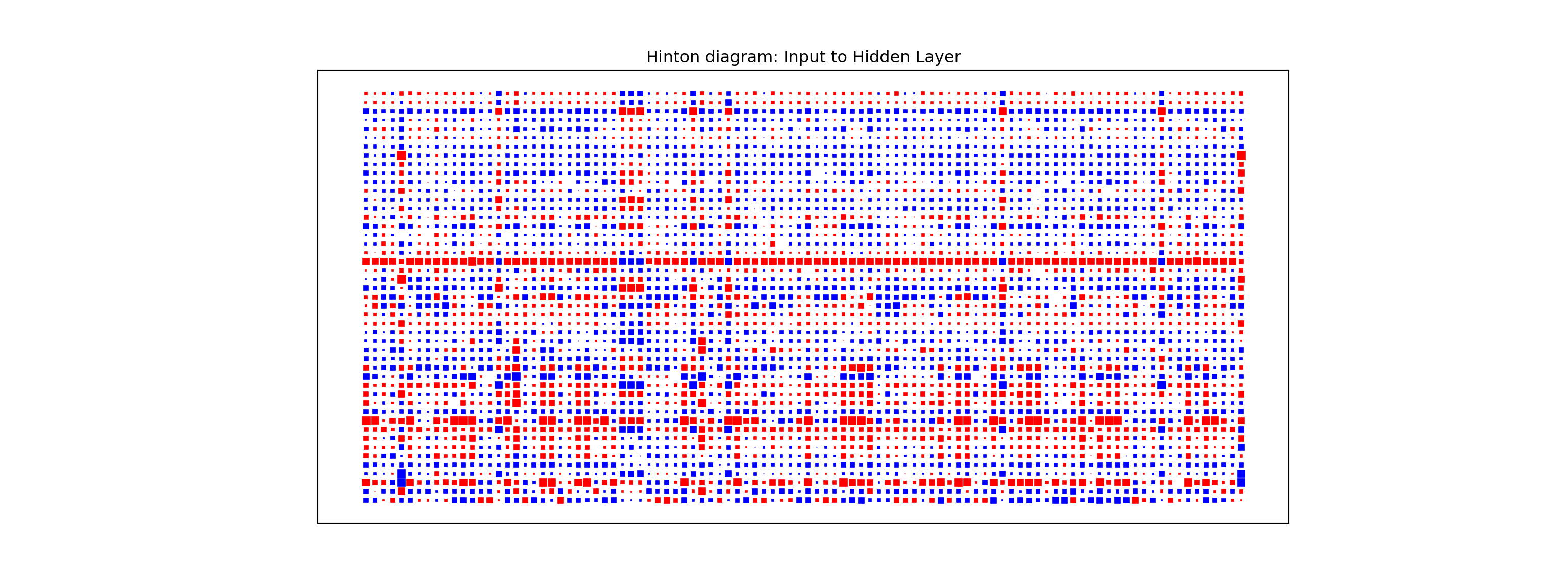
One way to visualize all the weights in a variable would be to use a Hinton diagram. This diagram is really only good for smaller numbers of variables. With hundreds of variables, a Hinton diagram becomes burdensome to view.
From the diagram above we see there are few instances of variables having low weights across all of the inputs to the hidden layers. The only ones we see are specific categories in a larger categorical variable. In this scenario, we would probably keep all of our variables.
Predictions
Models are nothing but potentially complicated formulas or rules. Once we determine the optimal model, we can score any new observations we want with the equation.
Scoring data does not mean that we are re-running the model/algorithm on this new data. It just means that we are asking the model for predictions on this new data - plugging the new data into the equation and recording the output. This means that our data must be in the same format as the data put into the model. Therefore, if you created any new variables, made any variable transformations, or imputed missing values, the same process must be taken with the new data you are about to score.
For this problem we will score our test dataset that we have previously set aside as we were building our model. The test dataset is for comparing final models and reporting final model metrics. Make sure that you do NOT go back and rebuild your model after you score the test dataset. This would no longer make the test dataset an honest assessment of how good your model is actually doing. That also means that we should NOT just build hundreds of iterations of our same model to compare to the test dataset. That would essentially be doing the same thing as going back and rebuilding the model as you would be letting the test dataset decide on your final model.
Without going into all of the same detail as before, the following code transforms the test dataset we originally created in the same way that we did for the training dataset by dropping necessary variables, making missing value imputations, and getting our same scaled data objects.
Code
predictors_test = test.drop(columns=['SalePrice'])ames_dummied = pd.get_dummies(ames, drop_first=True)test_ids = test.indextest_dummied = ames_dummied.loc[test_ids]predictors_test = test_dummied.astype(float)predictors_test = predictors_test.drop(['GarageType_Missing', 'GarageQual_Missing','GarageCond_Missing'], axis=1)# Impute Missing for Continuous Variablesnum_cols = predictors_test.select_dtypes(include='number').columnsfor col in num_cols:if predictors_test[col].isnull().any():# Create missing flag column predictors_test[f'{col}_was_missing'] = predictors_test[col].isnull().astype(int)# Impute with median median = predictors_test[col].median() predictors_test[col] = predictors_test[col].fillna(median)X_test = predictors_testy_test = test['SalePrice']y_test_log = np.log(test['SalePrice'])# Subset the DataFrame to selected featuresX_test_selected = X_test[selected_features].copy()X_test_selected = sm.add_constant(X_test_selected)scaler = StandardScaler()X_test_cont_scaled = scaler.fit_transform(X_test_selected[continuous_features])X_test_binary = X_test_selected[binary_features].valuesX_test_scaled = np.hstack((X_test_cont_scaled, X_test_binary))X_test_scaled_df = pd.DataFrame(X_test_scaled, columns=final_feature_order)
Now that our data is ready for scoring we can use the predict function on our model object we created with our decision tree. The only input to the predict function is the dataset we prepared for scoring.
From the sklearn.metrics package we have a variety of model metric functions. We will use the mean_absolute_error (MAE) and mean_absolute_percentage_error (MAPE) metrics like the ones we described in the section on Model Building.
From the above output we can see that the newly created neural network model is not as predictive as a lot of the previous models, but between the ridge and decision tree models.
Model
MAE
MAPE
Linear Regression
$18,160.24
11.36%
Ridge Regression
$19.572.19
12.25%
GAM
$18,154.31
11.40%
Decision Tree
$25,422.52
16.01%
Random Forest
$16,974.22
10.90%
XGBoost
$17,825.07
10.94%
EBM
$18,774.71
11.60%
Neural Network
$21,302.19
13.20%
To make sure that we are using the same test dataset between Python and R we will import our Python dataset here into R. There are a few variables that need to be renamed with the names function to work best in R.
test_cont_scaled <-scale( X_test_selected[, continuous_features, drop =FALSE], center =attr(X_cont_scaled, "scaled:center"), scale =attr(X_cont_scaled, "scaled:scale"))# Robust attribute stripping (for H2O compatibility)test_cont_scaled_df <-as.data.frame(test_cont_scaled)test_cont_scaled_df[] <-lapply(test_cont_scaled_df, unclass)# --- Step 3: Extract the remaining features (dummies) ---test_other_df <- X_test_selected[, remaining_cols, drop=FALSE]test_other_df[] <-lapply(test_other_df, as.numeric)# --- Step 4: Combine the scaled test data ---scaled_test_df <-cbind(test_cont_scaled_df, test_other_df)# Final coercion and conversion to H2OFramescaled_test_df[] <-lapply(scaled_test_df, as.numeric)
Now that our data is ready for scoring, we can use the h2o.predict function on our model object we created with our neural network. The only input to the h2o.predict function is the dataset we prepared for scoring, but that dataset must be converted into an h2o frame as before.
From the Metrics package we have a variety of model metric functions. We will use the mae (mean absolute error) and mape (mean absolute percentage error) metrics like the ones we described in the section on Model Building.
From the above output we can see that the newly created neural network model is not as predictive as a lot of the previous models, but around the ridge and decision tree models.
Model
MAE
MAPE
Linear Regression
$18,160.24
11.36%
Ridge Regression
$22,040.76
13.37%
GAM
$19,479.79
12.23%
Decision Tree
$22,934.49
13.92%
Random Forest
$16,864.85
10.77%
XGBoost
$18,285.01
11.37%
EBM
$18,801.94
11.64%
Neural Network
$20,615.96
13.45%
Summary
In summary, neural network models are good models to use for prediction, but explanation becomes more difficult and complex. Some of the advantages of using neural network models:
Used for both categorical and numeric target variables
Capable of modeling complex, nonlinear patterns
No assumptions about the data distributions
There are some disadvantages though:
No insights for variable importance
Extremely computationally intensive (very slow to train)
Tuning of parameters is burdensome
Prone to overfitting training data
Source Code
---title: "Neural Network Models"format: html: code-fold: show code-tools: trueengine: knitreditor: visual---```{r}#| include: false#| warning: false#| error: false#| message: falselibrary(reticulate)reticulate::use_condaenv("wfu_fall_ml", required =TRUE)``````{python}#| include: false#| warning: false#| error: false#| message: falsefrom sklearn.datasets import fetch_openmlimport pandas as pdfrom sklearn.feature_selection import SelectKBest, f_classifimport numpy as npimport matplotlib.pyplot as plt# Load Ames Housing datadata = fetch_openml(name="house_prices", as_frame=True)ames = data.frame# Remove Business Logic Variablesames = ames.drop(['Id', 'MSSubClass','Functional','MSZoning','Neighborhood', 'LandSlope','Condition2','OverallCond','RoofStyle','RoofMatl','Exterior1st','Exterior2nd','MasVnrType','MasVnrArea','ExterCond','BsmtCond','BsmtExposure','BsmtFinType1','BsmtFinSF1','BsmtFinType2','BsmtFinSF2','BsmtUnfSF','Electrical','LowQualFinSF','BsmtFullBath','BsmtHalfBath','KitchenAbvGr','GarageFinish','SaleType','SaleCondition'], axis=1)# Remove Missingness Variablesames = ames.drop(['PoolQC', 'MiscFeature','Alley', 'Fence'], axis=1)# Impute Missingness for Categorical Variablescat_cols = ames.select_dtypes(include=['object', 'category']).columnsames[cat_cols] = ames[cat_cols].fillna('Missing')# Remove Low Variability Variablesames = ames.drop(['Street', 'Utilities','Heating'], axis=1)# Train / Test Splitfrom sklearn.model_selection import train_test_splittrain, test = train_test_split(ames, test_size =0.25, random_state =1234)# Impute Missing for Continuous Variablesnum_cols = train.select_dtypes(include='number').columnsfor col in num_cols:if train[col].isnull().any():# Create missing flag column train[f'{col}_was_missing'] = train[col].isnull().astype(int)# Impute with median median = train[col].median() train[col] = train[col].fillna(median)# Prepare X and y Objectsimport statsmodels.api as smpredictors = train.drop(columns=['SalePrice'])predictors = pd.get_dummies(predictors, drop_first=True)predictors = predictors.astype(float)predictors = predictors.drop(['GarageType_Missing', 'GarageQual_Missing','GarageCond_Missing'], axis=1)X = predictorsy = train['SalePrice']y_log = np.log(train['SalePrice'])# Initial Variable Selectionselector = SelectKBest(score_func=f_classif, k='all') selector.fit(X, y)pval_df = pd.DataFrame({'Feature': X.columns,'F_score': selector.scores_,'p_value': selector.pvalues_})selected_features = pval_df[pval_df['p_value'] <0.009]['Feature']X_reduced = X[selected_features.tolist()]``````{r}#| include: false#| warning: false#| error: false#| message: falsetrain = py$traintest = py$testX_reduced = py$X_reducedy = py$yy_log = py$y_lognames(X_reduced)[names(X_reduced) =="1stFlrSF"] <-"FirstFlrSF"names(X_reduced)[names(X_reduced) =="2ndFlrSF"] <-"SecondFlrSF"names(X_reduced)[names(X_reduced) =="3SsnPorch"] <-"ThreeStoryPorch"```# Neural Network StructureNeural network models are considered "black-box" models because they are complex and hard to decipher relationships between predictor variables and the target variable. However, if the focus is on prediction, these models have the potential to model very complicated patterns in data sets with either continuous or categorical targets.The concept of neural networks was well received back in the 1980's. However, it didn't live up to expectations. Support vector machines (SVM's) overtook neural networks in the early 2000's as the popular "black-box" model. Recently there has been a revitalized growth of neural network models in image and visual recognition problems. There is now a lot of research in the area of neural networks and "deep learning" problems - recurrent, convolutional, feedforward, etc.Neural networks were originally proposed as a structure to mimic the human brain. We have since found out that the human brain is much more complex. However, the terminology is still the same. Neural networks are organized in a network of **neurons** (or nodes) through **layers**. The input variables are considered the neurons on the **bottom layer**. The output variable is considered the neuron on the **top layer**. The layers in between, called **hidden layers**, transform the input variables through non-linear methods to try and best model the output variable.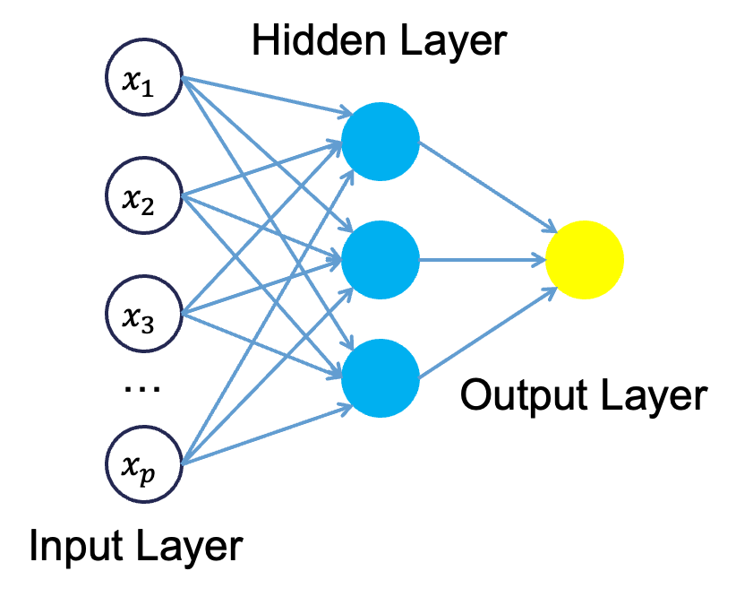{fig-align="center" width="4in"}All of the nonlinearities and complication of the variables get added to the model in the hidden layer. Each line in the above figure is a weight that connects one layer to the next and needs to be optimized. For example, the first variable $x_1$ is connected to all of the neurons (nodes) in the hidden layer with a separate weight.Let's look in more detail about what is happening inside the first neuron of the hidden layer.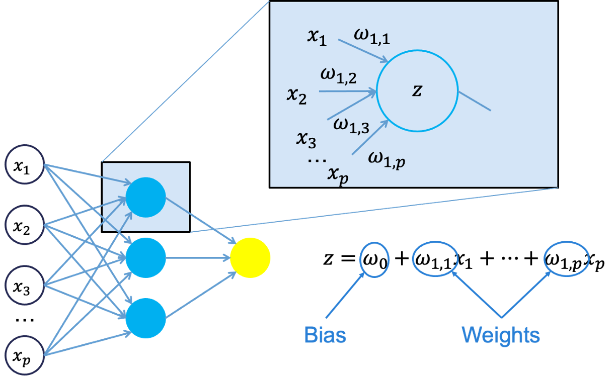{fig-align="center" width="7in"}Each of the variables is weighted coming into the neuron. These weights are combined with each of the variables in a linear combination with each other. With the linear combination we then perform a non-linear transformation.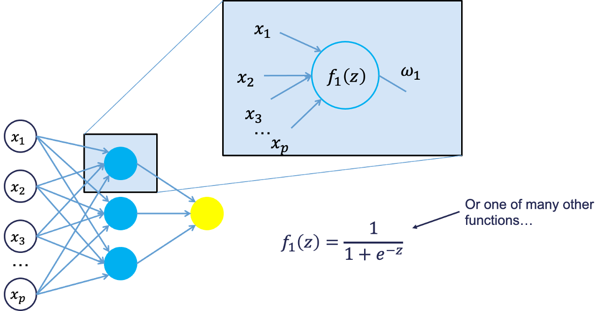{fig-align="center" width="7in"}There are many different nonlinear functions this could be. The main goal is to add complexity to the model. Each of the hidden nodes apply different weights to each of the input variables. This would mean that certain nonlinear relationships are highlighted for certain variables more than others. This is why we can have lots of neurons in the hidden layer so that many nonlinear relationships can be built.From there, each of the hidden layer neurons passes this nonlinear transformation to the next layer. If that next layer is another hidden layer, then the nonlinear transformations from each neuron in the first hidden layer are combined linearly in a weighted combination and another nonlinear transformation is applied to them. If the output layer is the next layer, then these nonlinear transformations are combined linearly in a weighted combination for a last time.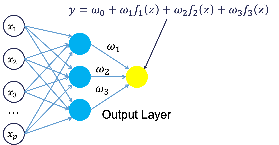{fig-align="center" width="5in"}Now we have the final prediction from our model. All of the weights that we have collected along the way are optimized to minimize sum of squared error. How this optimization is done is through a process called **backpropagation**.# BackpropagationBackpropagation is the process that is used to optimize the coefficients (weights) in the neural network. There are two main phases to backpropagation - a forward and backward phase.In the forward phase we have the following steps:1. Start with some initial weights (often random)2. Calculations pass through the network3. Predicted value computed.In the backward phase we have the following steps:1. Predicted value compared with actual value2. Work backward through the network to adjust weights to make the prediction better3. Repeat forward and backward until process convergesLet's look at a basic example with 3 neurons in the input layer, 2 neurons in the hidden layer, and one neuron in the output layer.{fig-align="center" width="5in"}Imagine 3 variables that take the values of 3, 4, and 5 with the corresponding weights being assigned to each line in the graph above. For the top neuron in the hidden layer you have $3\times 1 + 4 \times 0 + 5 \times 1 = 8$. The same process can be taken to get the bottom neuron. The hidden layer node values are then combined together (with no nonlinear transformation here) together to get the output layer.For the backward phase of backpropagation, let's imagine the true value of the target variable for this observation was 34. That means we have an error of 6 ($34-28=6$). We will now work our way back through the network changing the weights to make this prediction better. To see this process, let's use an even simpler example.Imagine you have a very simple equation, $y = \beta_1 x$. Now let's imagine you know that $y = 20$ and $x = 5$. However, you forgot how to do division! So you need backpropagation to find the value of $\beta_1$. To start with the forward phase, let's just randomly guess 3 for $\beta_1$ - our random starting point. Going through the network, we will use this guess of $\beta_1$ to get our final prediction of 15 ($=3 \times 5$). Since we know the true value of y is 20, we start with an error of $20-15 = 5$. Now we look at the backward phase of backpropagation. First we need the derivative of our loss function (sum of squared error). Without going through all the calculus details here, the derivative of the squared error at a single point is 2 multiplied by the error itself.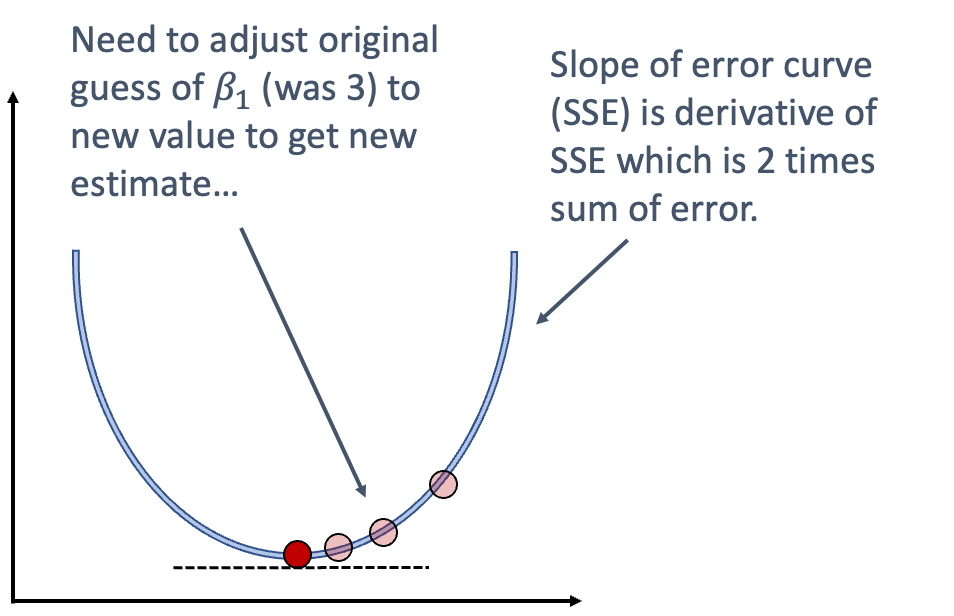{fig-align="center" width="5in"}The next step in baackpropagation is to adjust our original value of $\beta_1$ to account for this error and get a better estimate of $\beta_1$. To do this we multiply the slope of the error curve by the learning rate (set at some small constant like 0.05 to start) and then adjust the value of $\beta_1$.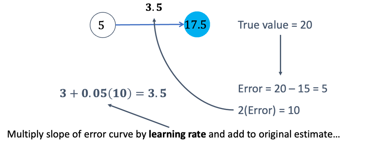{fig-align="center" width="6.5in"}Based on the figure above, our $\beta_1$ was 3, but has been adjusted to 3.5 based on the learning rate and slope of the loss function. Now we repeat the process and go forward through the network. This makes our prediction 17.5 instead of 15. This reduces our error from 5 to 2.5. The process goes backwards again to adjust the value of $\beta_1$ again.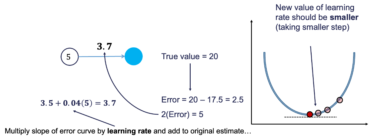{fig-align="center" width="8in"}We will still multiply the slope of the loss function (with our new error) by the learning rate. This learning rate should be adjusted to be smaller (from 0.05 to 0.04 above) to account for us being closer to the real answer. We will not detail how the backpropagation algorithm adjusts this learning rate here. However, this process will continue until some notion of convergence. In this example, it would continue until the slope estimate is 4 and the error would be 0 (its minimum).Although easy in idea, in practice this is much more complicated. To start, we have many more than just one single observation. So we have to calculate the error of all of the observations and get a notion of our loss function (sum of squared error in our example) across all the observations. The changing of the slope then impacts all of the observations, not just a single one. Next, we have more than one variable and weight to optimize at each step, making the process all the more complicated. Finally, this gets even more complicated as we add in many neurons in hidden layers so the algorithm has many layers to step backward through in its attempt to optimize the solution. These hidden layers also have complicated nonlinear functions, which make derivative calculations much more complicated than the simple example we had above. Luckily, this is what the computer helps do for us!# Tuning a Neural NetworkWhen it comes to tuning machine learning models like a neural network there are **many** options for tuning. **Cross-validation** should be included in each of these approaches. Two of the most common tuning approaches are:- Grid search- Bayesian optimizationGrid search algorithms look at a fixed grid of values for each parameter you can tune - called hyperparameters. This means that **every possible** combination of values no matter is they are good or bad as it doesn't learn from previous results. This is good for small samples with limited number of variables as it can be time consuming.Bayesian optimization on the other hand is typically less computationally expensive as a grid search approach. The Bayesian optimization approach starts with random values for each hyperparameter you need to tune. It then fits a probabilistic model (a type of sequential model-based optimization) that "learns" the relationship between the parameters and performance. This process tries to estimate which hyperparameters are likely to produce good results and point it in the "correct" direction for values of hyperparameters. The next step in the optimization essentially "learns" from the previous combinations of hyperparameters. This approach is much more valuable for large samples with large numbers of variables.Let's see how to build a neural network in each software!::: {.panel-tabset .nav-pills}## PythonAlthough not required, neural networks work best when data is scaled to a narrow range around 0. For bell shaped data, statistical z-score standardization would work:$$z_i = \frac{x_i - \bar{x}}{s_x}$$For severely asymmetric data, midrange standardization works better:$$\frac{x_i - midrange(x)}{0.5 \times range(x)} = \frac{x_i - \frac{\max(x) + \min(x)}{2}}{0.5 \times (\max(x) - \min(x))}$$For simplicity, we will use the `StandardScaler` function to standardize our data with the z-score method. However, we only want to standardize the continuous variables and not the binary ones.First, we will use the `nunique` function to identify how many unique values each variable has. Any variable with 2 or less unique values must be one of our categorical variables that we already dummy coded as binary. We then apply the `fit_transform` function to only the isolated continuous variables before recombining them with the binary variables using the `hstack` function from `numpy`. Once we put them back into a data frame with the `DataFrame` function we now have our data prepared for the neural network model.```{python}#| warning: false#| error: false#| message: falsefrom sklearn.preprocessing import StandardScaler unique_counts = X_reduced.nunique()continuous_features = unique_counts[unique_counts >2].index.tolist()binary_features = unique_counts[unique_counts ==2].index.tolist()final_feature_order = continuous_features + binary_featuresscaler = StandardScaler()X_cont_scaled = scaler.fit_transform(X_reduced[continuous_features])X_binary = X_reduced[binary_features].valuesX_scaled = np.hstack((X_cont_scaled, X_binary))X_scaled_df = pd.DataFrame(X_scaled, columns=final_feature_order)```Now that we have our data in a modelable format, we will then use the `MLPRegressor` function from the `sklearn.neural_network` packages to build out our neural network. The `MLPRegressor` function has expected inputs. The `hidden_layer_sizes =` option specifies how many neurons we want in each hidden layer. For multiple hidden layers, you would put multiple numbers. We will build one hidden layer with 100 neurons. We then use the `.fit` function with our standardized predictors and target variable to build out our model. The `activation = "relu"` option specifies we want the Rectified Linear Unity function. It is a simpler function than the logistic curve described above leading to less problems with convergence. It is defined as $\max(0, x)$. Therefore, any negative values are just taken as 0 while all positive values stay the same.```{python}#| warning: false#| error: false#| message: falsefrom sklearn.neural_network import MLPRegressornn_ames = MLPRegressor(max_iter =100000, solver ='adam', alpha =0.001, activation ='relu', hidden_layer_sizes = (100,), random_state =1234)nn_ames.fit(X_scaled_df, y)```In Python we will build and tune decision trees with both a grid search and Bayesian optimization approach to compare.To tune the `MLPRegressor` function we will go to the `GridSearchCV` function from `sklearn.model_selection`. In the `param_grid` for this iteration of the `GridSearchCV` function we will use the `hidden_layer_sizes`, `alpha`, and `activation` parameters. The `hidden_layer_sizes` parameter controls how many neurons are in our hidden layer. We will try out five values with one hidden layer and even try out a couple of two hidden layer neural networks. The `alpha` parameter is a regularization parameter to prevent overfitting. We will try two different activation functions - the ReLU and tanh functions. We will still keep our usual 10-fold cross-validation.```{python}#| warning: false#| error: false#| message: falsefrom sklearn.model_selection import GridSearchCV, KFoldparam_grid = {'alpha': [0.0001, 0.001, 0.01, 0.1],'activation': ['relu', 'tanh'],'hidden_layer_sizes': [(80,), (90,), (100,), (110,), (120,), (50, 20), (100, 50)]}cv = KFold(n_splits =10, shuffle =True, random_state =1234)nn = MLPRegressor(max_iter =100000, solver ='adam', random_state =1234, early_stopping =True)grid_search = GridSearchCV(estimator = nn, param_grid = param_grid, cv = cv, scoring ='neg_mean_squared_error')grid_search.fit(X_scaled_df, y)grid_search.best_params_```We can get the best parameters from using the `best_params_` element of the model object.Let's now build with Bayesian optimization. This involves slightly more complicated coding. First we must define our objective function where we similarly define our grid that we want to define. We will use the same hyperparameter values. We will still use the same `MLPRegressor` function as our grid search as well as the same `Kfold` function. The main differences come with the `create_study` function. This sets up the parameters previously defined with the objective. The `direction` option is used to tell the Bayesian optimization whether to maximize or minimize the outcome. The `sampler` option is where we control the seeding to make the optimization replicable. Inside of the `sampler` option we put in the `samplers.TPESampler` function with the seed set. Lastly, we use the `optimize` function with the defined objective on the `create_study` object. The `best_params` function gives us the optimal parameters from the Bayesian optimization.```{python}#| warning: false#| error: false#| message: falseimport optunafrom sklearn.model_selection import cross_val_scoreimport numpy as np# Step 1: Define the objective using a lambda so you keep your code flatdef objective(trial):# Define search space (equivalent to your param_grid) activation = trial.suggest_categorical('activation', ['relu', 'tanh']) alpha = trial.suggest_categorical('alpha', [0.0001, 0.001, 0.01, 0.1]) hidden_layer_sizes_str = trial.suggest_categorical('hidden_layer_sizes', ['80,', '90,', '100,', '110,', '120,', '50, 20', '100, 50']) hidden_layer_list = [int(s) for s in hidden_layer_sizes_str.split(',') if s.strip()] hidden_layer_sizes_tuple =tuple(hidden_layer_list)# Create the model with suggested parameters nn = MLPRegressor(max_iter =100000, solver ='adam', early_stopping =True, activation = activation, alpha = alpha, hidden_layer_sizes = hidden_layer_sizes_tuple, random_state =1234 )# 10-fold CV like your original cv = KFold(n_splits =10, shuffle =True, random_state =1234) scores = cross_val_score(nn, X_scaled_df, y, cv = cv, scoring ='neg_mean_squared_error') # or 'r2'return np.mean(scores)# Step 2: Run the optimizationstudy = optuna.create_study(direction ='maximize') # 'minimize' for error metricsstudy.optimize(objective, n_trials =20, show_progress_bar =True)# Step 3: Get the best hyperparametersprint("Best parameters:", study.best_params)print("Best score:", study.best_value)```We can see that having 2 hidden layers with 100 neurons in the first and 50 neurons in the second with an alpha parameter of 0.01 with the ReLU activation function is the optimal solution.```{python}nn_ames = MLPRegressor(max_iter =100000, solver ='adam', alpha =0.001, activation ='relu', hidden_layer_sizes = (100, 50), random_state =1234)nn_ames.fit(X_scaled_df, y)```## RAlthough not required, neural networks work best when data is scaled to a narrow range around 0. For bell shaped data, statistical z-score standardization would work:$$z_i = \frac{x_i-\bar{x}}{s_x}$$For severely asymmetric data, midrange standardization works better:$$\frac{x_i - midrange(x)}{0.5 \times range(x)} = \frac{x_i -\frac{\max(x)+\min(x)}{2}}{0.5 \times (\max(x) - \min(x))}$$For simplicity, we will use the `scale` function to standardize our data with the z-score method. However, we only want to standardize the continuous variables and not the binary ones.First, we will use the `unique` and `length` functions to identify how many unique values each variable has. Any variable with 2 or less unique values must be one of our categorical variables that we already dummy coded as binary. We then apply the `scale` function to only the isolated continuous variables before recombining them with the binary variables using the `cbind` function.```{r}#| warning: false#| error: false#| message: falseunique_counts <-sapply(X_reduced, function(x) length(unique(x)))continuous_features <-names(unique_counts[unique_counts >2])remaining_cols <-setdiff(colnames(X_reduced), continuous_features)X_cont_scaled <-scale(X_reduced[, continuous_features, drop =FALSE])X_cont_scaled_df <-as.data.frame(X_cont_scaled)X_cont_scaled_df[] <-lapply(X_cont_scaled_df, unclass)X_other_df <- X_reduced[, remaining_cols, drop=FALSE] X_other_df[] <-lapply(X_other_df, as.numeric)scaled_data_df <-cbind(X_cont_scaled_df, X_other_df)scaled_data_df$SalePrice <- y ```R has a much harder time developing neural networks than Python. To actually get neural networks with multiple hidden layers that we can use a grid search algorithm to tune, we need to download the `h2o` package. Also, to run the `h2o` package you need a Java Runtime Environment (JRE) installed on your computer.First, we need to convert our data frame into an H2O data frame using the `as.h2o` function. Once we do that we must isolate the predictor variables from the target variable. We use the `setdiff` function of the column names (`colnames`) to do so. From there we can now build our initial neural network with the `h2o.deeplearning` function. The inputs are rather straightforward with the inputs and target defined as `x =` and `y =` respectively. The H2O data frame is specified with the `training_frame` option. The hidden layer neuron count, activation function, and L2 penalty term as defined below as well.```{r}#| warning: false#| error: false#| message: falselibrary(h2o)h2o.init() scaled_data_df[] <-lapply(scaled_data_df, as.numeric)# Convert to H2OFrame object for modeling (required for H2O)h2o_frame <-as.h2o(scaled_data_df, destination_frame ="h2o_scaled_data")# Identify the predictor and response columns in the H2OFramepredictors <-setdiff(colnames(h2o_frame), "SalePrice")response <-"SalePrice"nn_ames_h2o <-h2o.deeplearning(x = predictors,y = response,training_frame = h2o_frame,hidden =100, activation ="Rectifier", l2 =0.001, epochs =100000, seed =1234,nfolds =0)# Print model summaryprint(nn_ames_h2o)```To be able to do a grid search in R with H2O the code becomes much more complicated. The sections are relatively straightforward if you break them down though. First, we define our grid of hyper parameters. We will try out five values with one hidden layer and even try out a couple of two hidden layer neural networks. The `l2` parameter is a regularization parameter to prevent overfitting. We will try two different activation functions - the ReLU and tanh functions. The search criteria defines how we want to perform the search. We will use the `strategy = 'Cartesian'` option to do an exhaustive grid search. We will still keep our usual 10-fold cross-validation.The `h2o.grid` function is where we combine these values together into the actual grid search algorithm. The remaining code after that is how we extract the best values from the grid to report the optimal neural network.```{r}#| warning: false#| error: false#| message: falsehyper_params <-list(hidden =list(c(80), c(90), c(100), c(110), c(120), c(50, 20), c(100, 50)),activation =c("Rectifier", "Tanh"), l2 =c(0.0001, 0.001, 0.01, 0.1))search_criteria <-list(strategy ="Cartesian")grid_search_h2o <-h2o.grid(algorithm ="deeplearning",grid_id ="mlp_grid",x = predictors,y = response,training_frame = h2o_frame,nfolds =10, epochs =10000, stopping_metric ="MSE", stopping_rounds =5, seed =1234,reproducible =TRUE,hyper_params = hyper_params,search_criteria = search_criteria)grid_results <-h2o.getGrid("mlp_grid", sort_by ="mse", decreasing =FALSE)print("--- Grid Search Complete. Best Models Ranked by MSE ---")print(grid_results)best_model_id <-h2o.getGrid(grid_search_h2o@grid_id, sort_by ="mse", decreasing =FALSE)@model_ids[[1]]best_nn_model <-h2o.getModel(best_model_id)best_params_R <-list(alpha = best_nn_model@parameters$l2, activation = best_nn_model@parameters$activation,hidden_layer_sizes = best_nn_model@parameters$hidden)print("--- Best Parameters Found (Equivalent to grid_search.best_params_) ---")print(best_params_R)```We can see that having 2 hidden layers with 100 neurons in the first and 50 neurons in the second with an alpha parameter of 0.001 with the Tanh activation function is the optimal solution.```{r}#| warning: false#| error: false#| message: falsenn_ames_h2o <-h2o.deeplearning(x = predictors,y = response,training_frame = h2o_frame,hidden =c(100,50), activation ="Tanh", l2 =0.001, epochs =100000, seed =1234,reproducible =TRUE,nfolds =0)# Print model summaryprint(nn_ames_h2o)```:::# Variable SelectionNeural networks typically do **not** care about variable selection. All variables are used by default in a complicated and mixed way. However, if you want to do variable selection, you can examine the weights for each variable. If all of the weights for a single variable are low, then you **might** consider deleting the variable, but again, it is typically not required.One way to visualize all the weights in a variable would be to use a Hinton diagram. This diagram is really only good for smaller numbers of variables. With hundreds of variables, a Hinton diagram becomes burdensome to view.```{python}#| warning: false#| error: false#| message: false#| echo: falseweights_input_hidden = nn_ames.coefs_[0] # shape: (n_features, n_hidden)weights_hidden_output = nn_ames.coefs_[1] # shape: (n_hidden, 1)import matplotlib.pyplot as pltimport numpy as npdef hinton(matrix, max_weight=None, ax=None):""" Draws Hinton diagram for a weight matrix with: - Blue for positive weights - Red for negative weights - White background """ ax = ax or plt.gca() ax.cla() ax.set_aspect('equal') ax.set_facecolor('white') ax.xaxis.set_major_locator(plt.NullLocator()) ax.yaxis.set_major_locator(plt.NullLocator())if max_weight isNone: max_weight =2** np.ceil(np.log2(np.abs(matrix).max()))for (y, x), w in np.ndenumerate(matrix): color ='blue'if w >0else'red' size = np.sqrt(abs(w) / max_weight) rect = plt.Rectangle([x - size /2, y - size /2], size, size, facecolor=color, edgecolor=color) ax.add_patch(rect) ax.autoscale_view() ax.invert_yaxis()plt.figure(figsize=(16, 6))hinton(weights_input_hidden)plt.title('Hinton diagram: Input to Hidden Layer')plt.show()```From the diagram above we see there are few instances of variables having low weights across all of the inputs to the hidden layers. The only ones we see are specific categories in a larger categorical variable. In this scenario, we would probably keep all of our variables.# PredictionsModels are nothing but potentially complicated formulas or rules. Once we determine the optimal model, we can **score** any new observations we want with the equation.Scoring data **does not** mean that we are re-running the model/algorithm on this new data. It just means that we are asking the model for predictions on this new data - plugging the new data into the equation and recording the output. This means that our data must be in the same format as the data put into the model. Therefore, if you created any new variables, made any variable transformations, or imputed missing values, the same process must be taken with the new data you are about to score.For this problem we will score our test dataset that we have previously set aside as we were building our model. The test dataset is for comparing final models and reporting final model metrics. Make sure that you do **NOT** go back and rebuild your model after you score the test dataset. This would no longer make the test dataset an honest assessment of how good your model is actually doing. That also means that we should **NOT** just build hundreds of iterations of our same model to compare to the test dataset. That would essentially be doing the same thing as going back and rebuilding the model as you would be letting the test dataset decide on your final model.Let's score our data in each software!::: {.panel-tabset .nav-pills}## PythonWithout going into all of the same detail as before, the following code transforms the test dataset we originally created in the same way that we did for the training dataset by dropping necessary variables, making missing value imputations, and getting our same scaled data objects.```{python}#| warning: false#| error: false#| message: falsepredictors_test = test.drop(columns=['SalePrice'])ames_dummied = pd.get_dummies(ames, drop_first=True)test_ids = test.indextest_dummied = ames_dummied.loc[test_ids]predictors_test = test_dummied.astype(float)predictors_test = predictors_test.drop(['GarageType_Missing', 'GarageQual_Missing','GarageCond_Missing'], axis=1)# Impute Missing for Continuous Variablesnum_cols = predictors_test.select_dtypes(include='number').columnsfor col in num_cols:if predictors_test[col].isnull().any():# Create missing flag column predictors_test[f'{col}_was_missing'] = predictors_test[col].isnull().astype(int)# Impute with median median = predictors_test[col].median() predictors_test[col] = predictors_test[col].fillna(median)X_test = predictors_testy_test = test['SalePrice']y_test_log = np.log(test['SalePrice'])# Subset the DataFrame to selected featuresX_test_selected = X_test[selected_features].copy()X_test_selected = sm.add_constant(X_test_selected)scaler = StandardScaler()X_test_cont_scaled = scaler.fit_transform(X_test_selected[continuous_features])X_test_binary = X_test_selected[binary_features].valuesX_test_scaled = np.hstack((X_test_cont_scaled, X_test_binary))X_test_scaled_df = pd.DataFrame(X_test_scaled, columns=final_feature_order)```Now that our data is ready for scoring we can use the `predict` function on our model object we created with our decision tree. The only input to the `predict` function is the dataset we prepared for scoring.From the `sklearn.metrics` package we have a variety of model metric functions. We will use the `mean_absolute_error` (MAE) and `mean_absolute_percentage_error` (MAPE) metrics like the ones we described in the section on Model Building.```{python}#| warning: false#| error: false#| message: falsefrom sklearn.metrics import mean_absolute_errorfrom sklearn.metrics import mean_absolute_percentage_errorpredictions = nn_ames.predict(X_scaled_df)nn_pred = nn_ames.predict(X_test_scaled_df)mae = mean_absolute_error(y_test, nn_pred)mape = mean_absolute_percentage_error(y_test, nn_pred)print(f"MAE: {mae:.2f}")print(f"MAPE: {mape:.2%}")```From the above output we can see that the newly created neural network model is not as predictive as a lot of the previous models, but between the ridge and decision tree models.| Model | MAE | MAPE ||:-----------------:|:-----------:|:------:|| Linear Regression | \$18,160.24 | 11.36% || Ridge Regression | \$19.572.19 | 12.25% || GAM | \$18,154.31 | 11.40% || Decision Tree | \$25,422.52 | 16.01% || Random Forest | \$16,974.22 | 10.90% || XGBoost | \$17,825.07 | 10.94% || EBM | \$18,774.71 | 11.60% || Neural Network | \$21,302.19 | 13.20% |## RTo make sure that we are using the same test dataset between Python and R we will import our Python dataset here into R. There are a few variables that need to be renamed with the `names` function to work best in R.```{r}#| warning: false#| error: false#| message: falsey_test <- py$y_testX_test_selected <- py$X_test_selectednames(X_test_selected)[names(X_test_selected) =="1stFlrSF"] <-"FirstFlrSF"names(X_test_selected)[names(X_test_selected) =="2ndFlrSF"] <-"SecondFlrSF"names(X_test_selected)[names(X_test_selected) =="3SsnPorch"] <-"ThreeStoryPorch"``````{r}#| warning: false#| error: false#| message: falsetest_cont_scaled <-scale( X_test_selected[, continuous_features, drop =FALSE], center =attr(X_cont_scaled, "scaled:center"), scale =attr(X_cont_scaled, "scaled:scale"))# Robust attribute stripping (for H2O compatibility)test_cont_scaled_df <-as.data.frame(test_cont_scaled)test_cont_scaled_df[] <-lapply(test_cont_scaled_df, unclass)# --- Step 3: Extract the remaining features (dummies) ---test_other_df <- X_test_selected[, remaining_cols, drop=FALSE]test_other_df[] <-lapply(test_other_df, as.numeric)# --- Step 4: Combine the scaled test data ---scaled_test_df <-cbind(test_cont_scaled_df, test_other_df)# Final coercion and conversion to H2OFramescaled_test_df[] <-lapply(scaled_test_df, as.numeric)```Now that our data is ready for scoring, we can use the `h2o.predict` function on our model object we created with our neural network. The only input to the `h2o.predict` function is the dataset we prepared for scoring, but that dataset must be converted into an `h2o` frame as before.From the `Metrics` package we have a variety of model metric functions. We will use the `mae` (mean absolute error) and `mape` (mean absolute percentage error) metrics like the ones we described in the section on Model Building.```{r}#| warning: false#| error: false#| message: falselibrary(Metrics)h2o_test_frame <-as.h2o(scaled_test_df, destination_frame ="h2o_scaled_test")predictions_h2o <-h2o.predict(object = best_nn_model, newdata = h2o_test_frame)nn_pred <-as.vector(predictions_h2o)mae_val <- Metrics::mae(y_test, as.numeric(nn_pred))mape_val <- Metrics::mape(y_test, as.numeric(nn_pred))cat(sprintf("MAE: %.2f\n", mae_val))cat(sprintf("MAPE: %.2f%%\n", mape_val *100))``````{r}#| warning: false#| error: false#| message: falseh2o.shutdown(prompt =FALSE)```From the above output we can see that the newly created neural network model is not as predictive as a lot of the previous models, but around the ridge and decision tree models.\| Model | MAE | MAPE ||:-----------------:|:-----------:|:------:|| Linear Regression | \$18,160.24 | 11.36% || Ridge Regression | \$22,040.76 | 13.37% || GAM | \$19,479.79 | 12.23% || Decision Tree | \$22,934.49 | 13.92% || Random Forest | \$16,864.85 | 10.77% || XGBoost | \$18,285.01 | 11.37% || EBM | \$18,801.94 | 11.64% || Neural Network | \$20,615.96 | 13.45% |:::# SummaryIn summary, neural network models are good models to use for prediction, but explanation becomes more difficult and complex. Some of the advantages of using neural network models:- Used for both categorical and numeric target variables- Capable of modeling complex, nonlinear patterns- No assumptions about the data distributionsThere are some disadvantages though:- No insights for variable importance- Extremely computationally intensive (**very slow** to train)- Tuning of parameters is burdensome- Prone to overfitting training data