Code
ar2 %>%
  gg_tsdisplay(Y, lag = 12, plot_type='partial')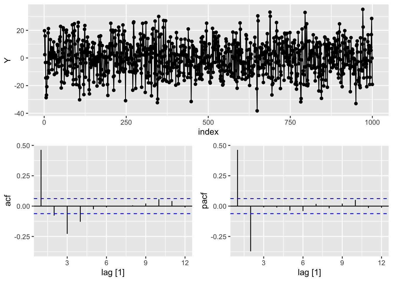
Once the data is made stationary (or if the data is stationary by default) we can move into a class of models called stationary models. One of the common stationary models, is the autoregressive (AR) model.
Often you can forecast a series based solely on the past values of the data. We are going to start by focusing on the most basic case with only one lag value of \(Y_t\), called the AR(1) model:
\[ Y_t = \omega + \phi Y_{t-1} + e_t \]
where \(e_t\) is the error remaining in the model and assumed to by white noise as defined in the previous section on stationarity.
With the AR(1) model, this relationship between t and t-1 exists for all one time period differences across the dataset. Therefore, we can recursively solve for \(Y_t\). We do this because we know that the equation for \(Y_{t-1}\) is:
\[ Y_{t-1} = \omega + \phi Y_{t-2} + e_t \]
By plugging this equation into the original equation of \(Y_t\) we have:
\[ Y_t = \omega + \phi (\omega + \phi Y_{t-2} + e_{t-1}) + e_t \]
\[ Y_t = \omega^* + \phi^2 Y_{t-2} + \phi e_{t-1} + e_t \]
We also know the equation for \(Y_{t-2}\) is the following:
\[ Y_{t-2} = \omega + \phi Y_{t-3} + e_{t-2} \]
By plugging this equation in the recursive solution of \(Y_t\) above we get:
\[ Y_t = \omega^* + \phi^2 (\omega + \phi Y_{t-3} + e_{t-2}) + \phi e_{t-1} + e_t \]
\[ Y_t = \omega^{**} + \phi^3 Y_{t-3} + \phi^2 e_{t-2} + \phi e_{t-1} + e_t \]
We can continue this process until we get back to the first data point at \(t=1\) in our dataset.
\[ Y_t = \frac{\omega}{1 - \phi} + \phi^t Y_1 + \phi^{t-1} e_2 + \phi^{t-2} e_3 + \cdots + e_t \]
We can see that the effect of shocks that happened long ago has little effect on the present value, \(Y_t\), as long as the value for \(|\phi| < 1\). This goes back to our idea of this being a stationary model. The dependence of previous observations declines over time. This means that although \(Y_1\) has some effect at \(Y_t\), that effect gets smaller the further away in time we are from \(Y_1\).
For data that follows an AR(1) structure, there are specific patterns we see in the autocorrelation and partial autocorrelation function. For a review of these functions, please see the previous section on correlation functions. With an AR(1) structure to our data, the autocorrelation function (ACF) decreases exponentially as the number of lags increases. The partial autocorrelation function (PACF) has a significant spike at the number one lag in the model, followed by nothing after.
Let’s imagine our data follows the following AR(1) process:
\[ Y_t = 0 + 0.8 Y_{t-1} + e_t \]
The following plots would be be the ACF and PACF of the data that follows the above structure.

In the ACF plot on the left above, the first lag takes a value of \(0.8\). The second lag is \(0.8^2 = 0.64\). The third lag is \(0.8^3 = 0.512\) and the pattern continues from there to get smaller as the lags go further back in time. For the PACF plot, the first lag takes a value of \(0.8\). The rest of the lags in the PACF take the value of zero because after accounting for the first lag, the remaining lags have no impact on the current time period.
This autoregressive model can be extended to include \(p\) lags instead of just one lag:
\[ Y_t = \omega + \phi_1 Y_{t-1} + \phi_2 Y_{t-2} + \cdots + \phi_p Y_{t-p} + e_t \]
With an autoregressive structure to our data, the autocorrelation function (ACF) decreases exponentially in the long run as the number of lags increases but with a variety of patterns. The partial autocorrelation function (PACF) has a significant spike up to \(p\) lags in the model, followed by nothing after.
The stationarity assumption still holds for this model as well with a slightly different requirement. Let’s look back at the AR(1) model after we recursively built it back into time:
\[ Y_t = \frac{\omega}{1 - \phi} + \phi^t Y_1 + \phi^{t-1} e_2 + \phi^{t-2} e_3 + \cdots + e_t \]
Look at the intercept in the previous equation. If the value of \(\phi = 1\), then the intercept would be \(\infty\). This is why we required \(|\phi| < 1\) for our model to be a stationary model.
Let’s now expand the AR(2) model back into time and see what it would look like:
\[ Y_t = \frac{\omega}{1 - \phi_1 - \phi_2} + \cdots + e_t \]
where \(\phi_1\) and \(\phi_2\) are the coefficients on the first two lags of \(Y_t\). In this scenario we would need \(|\phi_1 + \phi_2|<1\) for the model to have have an intercept take the value of \(\infty\). That is our stationarity condition for the AR(2) model.
Let’s now expand the AR(p) model back into time and see what it would look like:
\[ Y_t = \frac{\omega}{1 - \phi_1 - \cdots - \phi_p} + \cdots + e_t \]
where \(\phi_1\) through \(\phi_p\) are the coefficients on the first \(p\) lags of \(Y_t\). In this scenario we would need \(|\phi_1 + \cdots + \phi_p|<1\) for the model to have have an intercept take the value of \(\infty\). That is our stationarity condition for the AR(p) model.
Let’s see how to build this in each of our softwares!
We need to use a different dataset that is much more situated for an autoregressive model instead of the US airlines passengers dataset we have used up until this point. For this we will load a dataset that specifically follows an autoregressive structure. Let’s explore the dataset with the gg_tsdisplay function. Specifically, we will look at the Y variable across 12 lags. The plot_type = 'partial' option shows us the ACF and PACF for the variable.
ar2 %>%
gg_tsdisplay(Y, lag = 12, plot_type='partial')
From the plots above we can see early spikes in the ACF that tail off as we go further back in time in terms of lags. However, the PACF plot only has two spikes before all the remaining spikes are essentially 0. To see these patterns better we can use the Acf and Pacf functions from the forecast package to individually plot the ACF and PACF respectively.
forecast::Acf(ar2$Y, lag = 12, main = "ACF Plot")Registered S3 method overwritten by 'quantmod':
method from
as.zoo.data.frame zoo 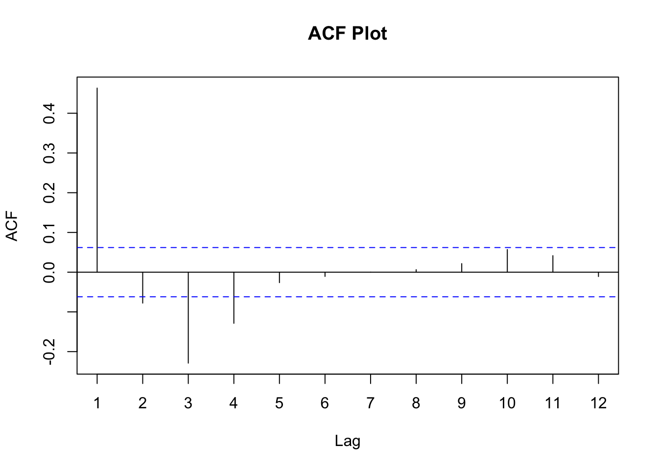
forecast::Pacf(ar2$Y, lag = 12, main = "PACF Plot")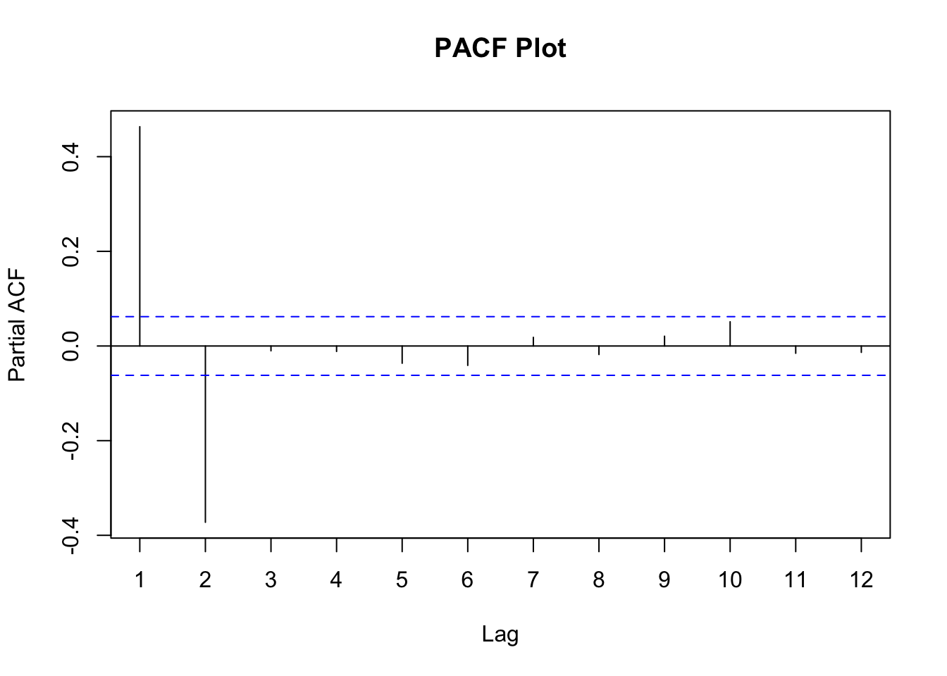
From what we saw earlier, a pattern in the PACF where there are two significant spikes followed by no correlation implies we should model our data with an AR(2) model. We can use the model function (from the fable package) with the ARIMA function to specify an autoregressive model. With the formula input to the ARIMA function we have our target variable of Y along with an intercept (represented by the 1) and the pdq function to specify the number of lags of the autoregressive term. The first term is the number of autoregressive lags which we set to 2. The second term is the number of single differences which we set to 0 since our data is already stationary. The last term is the number of lags in the moving average piece which we will talk about in the next section. Lastly, we use the report function to get a summary of the output from the model.
model_AR <- ar2 %>%
  model(
    ARIMA(Y ~ 1 + pdq(2,0,0))
    )

report(model_AR)
Series: Y
Model: ARIMA(2,0,0) w/ mean
Coefficients:
ar1 ar2 constant
0.6406 -0.3760 -0.1008
s.e. 0.0294 0.0294 0.3079
sigma^2 estimated as 95.07: log likelihood=-3695.01
AIC=7398.03 AICc=7398.07 BIC=7417.66What we can see form the above output is the values of \(\phi_1\) and \(\phi_2\) along with the intercept, \(\omega\).
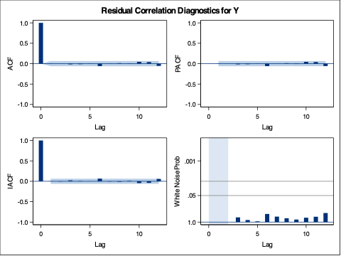
To see if we removed all of the correlation from our data we can examine the residuals using the gg_tsresiduals function. To get a sense of whether these residuals are white noise we can use the features function with the ljung_box option. We will calculate this test for 12 lags with dof = 2 since our model had two coefficients.
model_AR %>%
  gg_tsresiduals()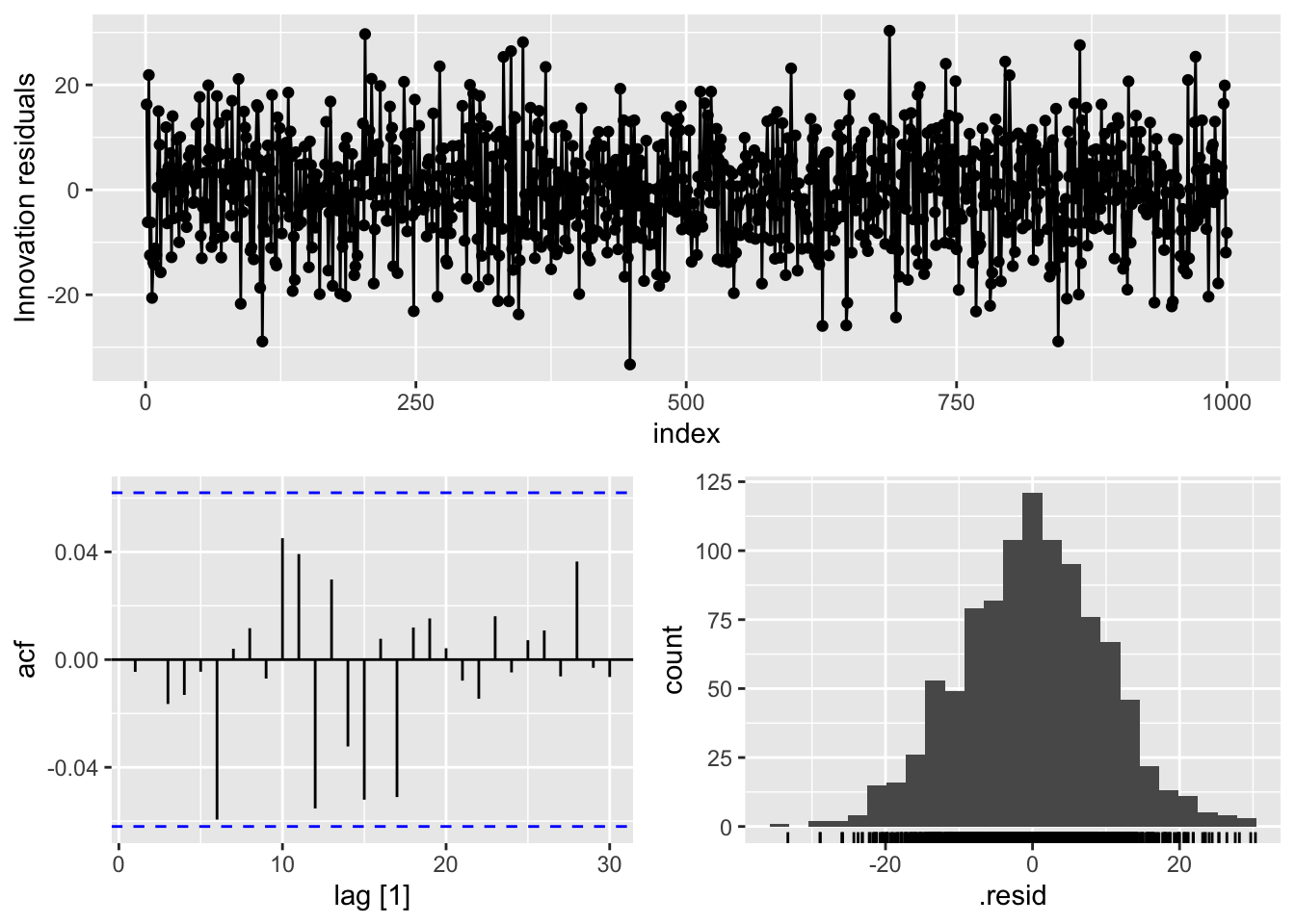
augment(model_AR) %>%
  features(.innov, ljung_box, lag = 12, dof = 2)
# A tibble: 1 × 3
.model lb_stat lb_pvalue
<chr> <dbl> <dbl>
1 ARIMA(Y ~ 1 + pdq(2, 0, 0)) 11.0 0.360Based on the picture above we can see that we have residuals that see to have no correlation to them. The p-value from the Ljung-Box test shows that we have white noise statistically.
We need to use a different dataset that is much more situated for an autoregressive model instead of the US airlines passengers dataset we have used up until this point. For this we will load a dataset that specifically follows an autoregressive structure. Let’s explore the dataset by looking at the ACF and PACF functions. To see these patterns better we can use the plot_acf and plot_pacf functions from the statsmodels.api package to individually plot the ACF and PACF respectively.
import statsmodels.api as sm

sm.graphics.tsa.plot_acf(ar2['y'],  lags = 12)

plt.show();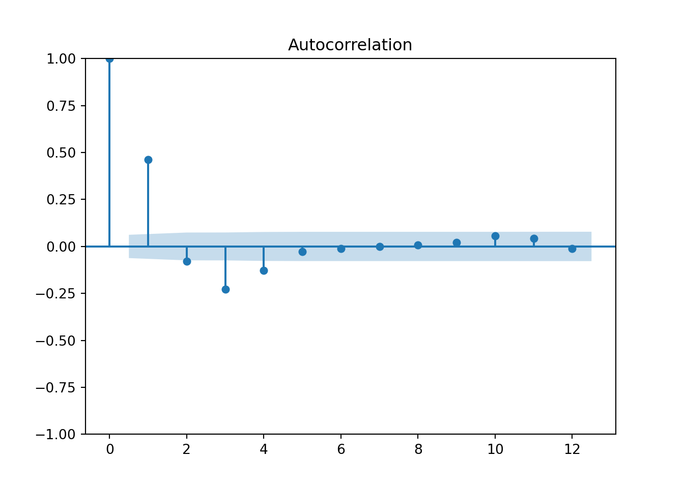
sm.graphics.tsa.plot_pacf(ar2['y'],  lags = 12)

plt.show();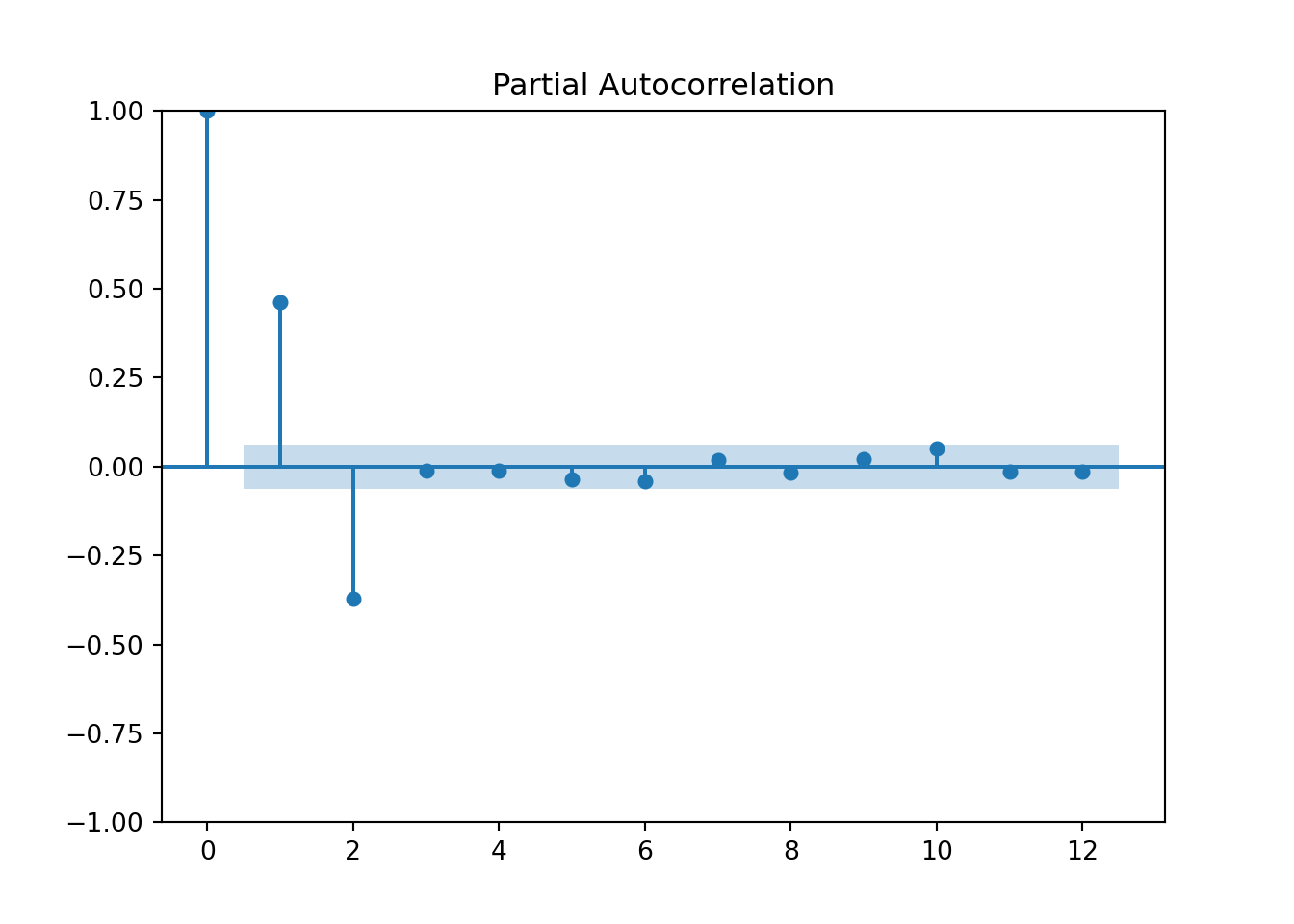
From the plots above we can see early spikes in the ACF that tail off as we go further back in time in terms of lags. However, the PACF plot only has two spikes before all the remaining spikes are essentially 0.
From what we saw earlier, a pattern in the PACF where there are two significant spikes followed by no correlation implies we should model our data with an AR(2) model. We can use the StatsForecast function with the ARIMA function to specify an autoregressive model. With the ARIMA function we have our target variable of Y and the order option to specify the number of lags of the autoregressive term. The first term is the number of autoregressive lags which we set to 2. The second term is the number of single differences which we set to 0 since our data is already stationary. The last term is the number of lags in the moving average piece which we will talk about in the next section. By using the .fit function we can build our AR(2) model. Lastly, we use the .fitted_[0][0].model_.get('coef') function to get a summary of the coefficients from the model.
from statsforecast import StatsForecast
from statsforecast.models import ARIMA

model_AR = StatsForecast(models = [ARIMA(order = (2, 0, 0))], freq = 1)
model_AR.fit(df = ar2)StatsForecast(models=[ARIMA])model_AR.fitted_[0][0].model_.get("coef"){'ar1': 0.6405515863182623, 'ar2': -0.3759502661066081, 'intercept': -0.13720809553198104}What we can see form the above output is the values of \(\phi_1\) and \(\phi_2\) along with the intercept, \(\omega\).
To see if we removed all of the correlation from our data we can examine the residuals. To get a sense of whether these residuals are white noise we can use the acorr_ljungbox function. We will calculate this test for 12 lags with model_df = 2 since our model had two coefficients.
sm.stats.acorr_ljungbox(model_AR.fitted_[0][0].model_.get("residuals"), lags = [12], model_df = 2) lb_stat lb_pvalue
12 10.964395 0.360299Based on the picture above we can see that we have residuals that see to have no correlation to them. The p-value from the Ljung-Box test shows that we have white noise statistically.
We need to use a different dataset that is much more situated for an autoregressive model instead of the US airlines passengers dataset we have used up until this point. For this we will load a dataset that specifically follows an autoregressive structure. Let’s explore the dataset by looking at the ACF and PACF functions. We can use the PROC ARIMA procedure in SAS to view the ACF and PACF functions. The plot = all option gives us the necessary plots. The IDENTIFY statement is where we specify the variable of interest using the var = option. We will look at the target variable Y for up to 12 lags.
proc arima data = ar2 plot = all;
    identify var = Y nlag = 12;
run;
From the plots above we can see early spikes in the ACF that tail off as we go further back in time in terms of lags. However, the PACF plot only has two spikes before all the remaining spikes are essentially 0.
From what we saw earlier, a pattern in the PACF where there are two significant spikes followed by no correlation implies we should model our data with an AR(2) model. We can use the same PROC ARIMA procedure to specify an autoregressive model too. We still need the same IDENTIFY statement to identify the target variable of Y. The ESTIMATE statement is used to specify the number of lags of the autoregressive term using the p = option. We set this number of autoregressive lags to 2. The last option we use is the method = ML option to specify building our model using maximum likelihood estimation.
proc arima data = ar2 plot = all;
    identify var = Y nlag = 12;
    estimate p = 2 method = ML;
run;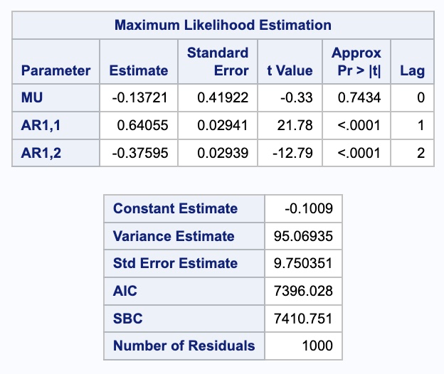
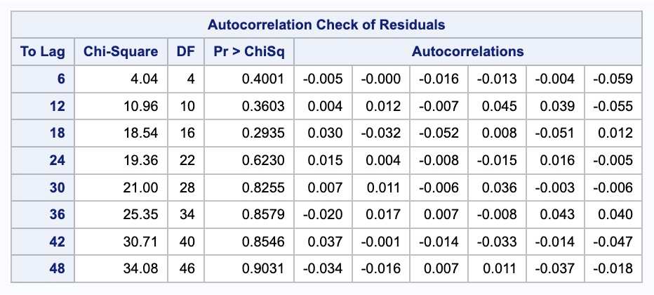
What we can see form the above output is the values of \(\phi_1\) and \(\phi_2\) along with the intercept, \(\omega\). To see if we removed all of the correlation from our data we can examine the residual output from above as well. To get a sense of whether these residuals are white noise we can use the p-values in the autocorrelation check of residuals table. This shows us that our residuals are white noise. This can also be seen in the white noise plot above too. That white noise plot above is a little hard to grasp at first. The bars more represent the test statistics than the p-values. Larger test statistics would lead to smaller p-values. The alpha levels are marked on the y-axis to show you if the test statistic is too large.