Time Series and Forecasting
Instructor: Dr. Aric LaBarr
Introduction
Time series and forecasting are a fundamental concepts and technique for data science and analytics. However, time series data is different than traditional data. Time series data is a set of ordered data values that we observe at (ideally) successive points in time. Think of time series as the evolution of a variable over time.
Quick Summary
Data Structure
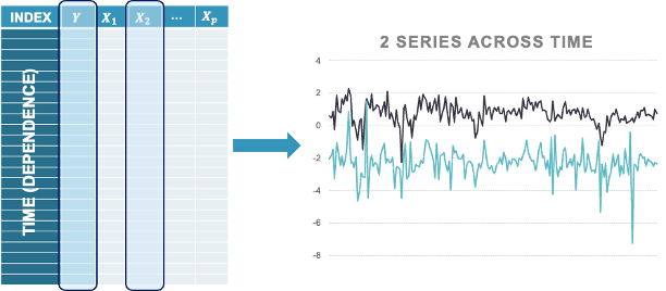
This structure is different than the typical cross-sectional data set you’re probably used to working with. Cross-sectional data are a set of data values observed at a fixed point in time, or where time is of no significance. An example of this is shown below:
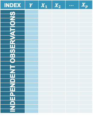
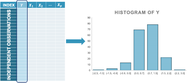
Your data typically looks like the above table. You have some indexing variable as well as a variable of interest that we will call Y. You also have a variety of other variables that may influence that variable of interest which we will denote with X’s. This indexing variable is an independent collection of observations. For example, they could be independent stores, independent products, or independent customers. This assumption of independence influences how we explore cross-sectional data. When exploring the variable of interest, we use histograms so we can visualize how spread out this variable is as well as what are common values of this variable.
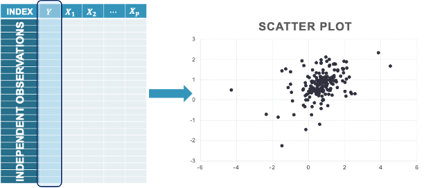
If we want to understand the relationship that our variable of interest may have with our other variables (X’s), we can look at scatter plots instead. For example, as Y increases, we could see that one of the X’s also tends to increase as well.
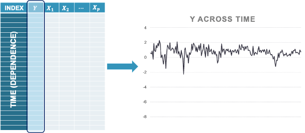
With time series data, our indexing variable changes. The indexing is actually time itself, which means there is a dependence structure you are observing as the variable of interest evolves over time. Therefore, Y is no longer an independent collection of observations, but a collection of successive points instead. This means we have to be really careful with missing data points. Having missing data in cross-sectional data may not impact the observations around it due to independence. Here, without that independence, missing values impact the observations around them.

If we look at the variable of interest across time, a histogram doesn’t provide the full picture of what we want to see with our variable. Instead, we view our variables across time when we have time series data. Where the variable is located as well as its spread may change as time goes on. For example, our variable is more spread out early in time as compared to later in the series. You can even make an argument that the center of the variable is slightly decreasing as time goes on.
It is the same with the target variable’s relationship with the X’s as well. We no longer care just about the values of a specific X and Y, but how they relate across time. For example, do the series spike at the same times? Do they both tend to decrease? If X spikes now, does Y spike later? These are the kinds of things we can explore when visualizing the data over time.
Uses for Time Series
Even though time series data is structured different, we typically use time series for similar purposes that we have for cross-sectional data - explanation or prediction / forecasting. Look at the examples below:
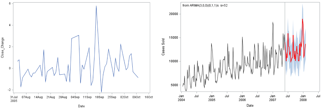
In the picture on the left, we see Southwest Airline stock during a few months of 2005. We see this large spike in the data. Looking at other data, we see that Delta Airline declared bankruptcy on that day. In the picture on the right, we have sales over years. Our goal is to provide a forecast of future sales to better plan.
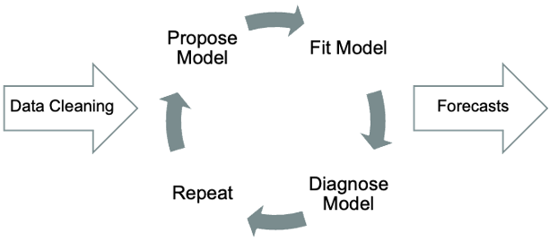
With either purpose for your analysis, the process for time series / forecasting stays the same:
Data Cleaning
Propose Model
Fit Model
Diagnose Model
Repeat steps 2 - 4 until satisfied
Forecast / Explain
Once the data is cleaned and ready for analysis, we move into the model building phase of the project. This model building phase is typically circular in nature where we try many different approaches and find the one that works best for our goals. Once we have that final model, we move to our outcome of either forecasting or explanation.
This website contains information on how to perform time series and forecasting and all of its components in R, Python, and SAS. In each section you are able to toggle back and forth between the code and output you desire to view.
The libraries for R and Python will be loaded as we go throughout the code. This isn’t needed for the SAS sections of the code.