Exponential Smoothing Models

Quick Summary

Time Dependency

Time series data relies on the assumption that the observations at a certain time point depend on previous observations in time. The most extreme versions of this assumption is the naive model and the average model. The naive model assumes that any prediction in the future (h observations) is just the latest known value at the current time, t:

\[ \hat{Y}_{t+h} = Y_t \]

The average model is the other extreme that assumes that any prediction in the future (h observations) are the equally weighted average of all of the data in the past:

\[ \hat{Y}_{t+h} = \frac{1}{T} \sum^T_{t=1} Y_t \]

Obviously, a better approach might be to use all of the data (like the average model) but emphasize more recent data (like the naive model) more heavily. The is the approach of the class of models called exponential smoothing models (ESMs). In exponential smoothing models the weights on the observations emphasize the most recent data, requires only estimating a few parameters, and are simple and easy to implement.

There are many different types of exponential smoothing models. Here we will discuss three common types:

Single (or Simple) ESM
Linear / Holt (incorporating trend) ESM
Holt-Winters (incorporating trend and seasonality) ESM

Single Exponential Smoothing

In single exponential smoothing we apply a weighting scheme that decreases exponentially the further back in time we go:

\[ \hat{Y}_{t+1} = \theta Y_t + \theta (1 - \theta) Y_{t-1} + \theta (1 - \theta)^2 Y_{t-2} + \theta(1 - \theta)^3 Y_{t-3} + \cdots \]

where $0 \le \theta \le 1$. The previous equation for the single exponential smoothing model can be written more simply as the following:

\[ \hat{Y}_{t+1} = \theta Y_t + (1 - \theta)Y_t \]

The single exponential smoothing model can also be written in component form:

\[ \hat{Y}_{t+1} = L_t \] \[ L_t = \theta Y_t + (1 - \theta)L_{t-1} \]

where the first equation is the forecast equation and the second equation is the level equation.

The larger the value of $\theta$, the more that the most recent observation is emphasized as shown by the chart below.

The optimal value of $\theta$ is the value that minimizes the one-step ahead forecast errors using the sum of these squared errors:

\[ SSE = \sum_{t=1}^T (Y_t - \hat{Y}_t)^2 \]

Visually, this looks like the following picture:

where each of the dashed lines in the plot above would be squared and summed together. That value of $\theta$ that minimizes that quantity is the optimal value. The only downside of optimizing only for the next time period is that you only get a forecast that is one value in the future. Any forecast beyond the initial point is the exact same as the initially forecasted point.

Some statistical software will report statistical tests for the $\theta$ parameter, but not everyone considers the results of these tests because the model was never derived and designed with statistical distributions and significance in mind.

Seasonal Exponential Smoothing

Exponential smoothing models can also account for seasonal factors. In seasonal exponential smoothing models, weights decay with respect to the seasonal factor:

There are multiple ways to incorporate a seasonal effect in the exponential smoothing framework.

Winters Additive Seasonal ESM
Winters Multiplicative Seasonal ESM
Holt Winters Additive Seasonal ESM
Holt Winters Multiplicative Seasonal ESM

Winters Seasonal Exponential Smoothing

If your data is seasonal in structure, but has no trend, then the Winters seasonal exponential smoothing model is a good model to use. Instead of the trend component that we saw in the Holt exponential smoothing model, the Winters model includes a seasonal component. Similar to what we saw with time series decomposition, the seasonal term can have an additive or multiplicative structure:

Additive Seasonal Component:

\[ \hat{Y}_{t+k} = L_t + S_{t-p+k} \] \[ L_t = \theta (Y_t - S_{t-p}) + (1 - \theta)L_{t-1} \] \[ S_t = \delta(Y_t - L_t) + (1 - \delta)S_{t-p} \]

Multiplicative Seasonal Component:

\[ \hat{Y}_{t+k} = L_t \times S_{t-p+k} \] \[ L_t = \theta (Y_t / S_{t-p}) + (1 - \theta)L_{t-1} \] \[ S_t = \delta(Y_t / L_t) + (1 - \delta)S_{t-p} \]

where $k$ is the number of observations to be forecasted. From the above equations we can see that the only difference is that we either add in the seasonal component, or multiply in the seasonal component. The optimal values of $\theta$ and $\delta$ are determined by minimizing the sum of squared errors of the one-step ahead forecast error. However, with the seasonal component, one-step ahead is one season ahead which means the model is optimized to predict one season into the future, instead of just one observation.

Holt Winters Seasonal Exponential Smoothing

If your data is seasonal in structure, and has a trend, then the Holt Winters (Triple) seasonal exponential smoothing model is a good model to use. Instead addition to the trend component that we saw in the Holt exponential smoothing model, the Holt Winters model includes a seasonal component as well. Similar to what we saw with time series decomposition, the seasonal term can have an additive or multiplicative structure:

Additive Seasonal Component:

\[ \hat{Y}_{t+k} = L_t + k T_t + S_{t-p+k} \] \[ L_t = \theta (Y_t - S_{t-p}) + (1 - \theta)(L_{t-1} + T_{t-1}) \] \[ T_t = \gamma(L_t - L_{t-1}) + (1 - \gamma) T_{t-1} \] \[ S_t = \delta(Y_t - L_t) + (1 - \delta)S_{t-p} \]

Multiplicative Seasonal Component:

\[ \hat{Y}_{t+k} = (L_t + k T_t) \times S_{t-p+k} \] \[ L_t = \theta (Y_t / S_{t-p}) + (1 - \theta)(L_{t-1} + T_{t-1}) \] \[ T_t = \gamma(L_t - L_{t-1}) + (1 - \gamma) T_{t-1} \] \[ S_t = \delta(Y_t / L_t) + (1 - \delta)S_{t-p} \]

where $k$ is the number of observations to be forecasted. From the above equations we can see that the only difference is that we either add in the seasonal component, or multiply in the seasonal component. The optimal values of $\theta$, $\gamma$, and $\delta$ are determined by minimizing the sum of squared errors of the one-step ahead forecast error. However, with the seasonal component, one-step ahead is one season ahead which means the model is optimized to predict one season into the future along a trend line, instead of just one observation.

Since our data has both a trend and seasonal component, we will build a Holt Winters Exponential smoothing model.

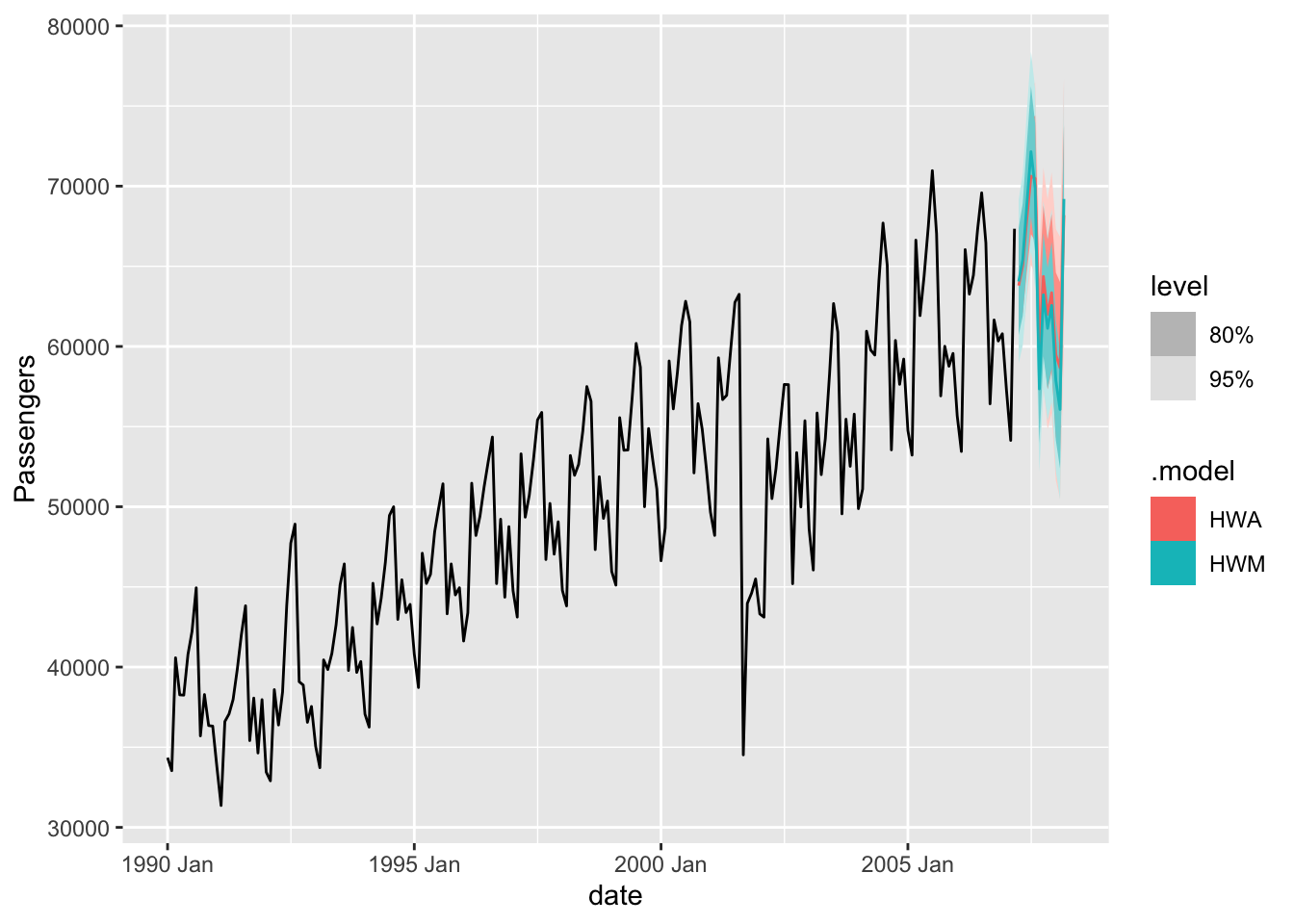
Let’s see how to do that in all of our software!

To build out our exponential smoothing models, we will still use the model function on our training dataset. The model function can specify multiple models to build at once for comparing against each other. To build an exponential smoothing model we use the ETS function in the model function. Within the ETS function we write a formula specifying the model we want. Here we have our target variable, Passengers, on the left hand side of the ~ followed by our components from the ESM’s. For the first model (which we name HWM, we will build a multiplicative Holt Winters model. For the multiplicative Holt Winters we specify the additive trend term (trend("A")), and the multiplicative seasonal term (season("M") and error("M")). Although the error and season don’t have to match, that would be a different structure than the Holt Winters model. The same thing can be done with our second model named HWA. We use the ETS function still, but instead we put in an additive season and error component to get the additive Holt Winters model. It is easy to see how you could get other exponential smoothing models we have discussed by removing different components from the formula.

From there we will use the glance function to look at some basic summaries about each model to compare how well they did with our training data. We then use the forecast function from the fabletools package to forecast out 12 observations (h = 12) in the future. We then finish up with the autoplot function to plot the forecasts from each of our models.

Code

model_HW <- train %>%
  model( 
    HWM = ETS(Passengers ~ error("M") + trend("A") + season("M")),
    HWA = ETS(Passengers ~ error("A") + trend("A") + season("A"))
  )

glance(model_HW)

# A tibble: 2 × 9
  .model        sigma2 log_lik   AIC  AICc   BIC      MSE     AMSE       MAE
  <chr>          <dbl>   <dbl> <dbl> <dbl> <dbl>    <dbl>    <dbl>     <dbl>
1 HWM          0.00165  -2116. 4267. 4270. 4324. 3879625. 4816426.    0.0240
2 HWA    3962758.       -2116. 4266. 4269. 4323. 3656458. 5008157. 1186.

Code

model_HW_for <- model_HW %>%
  fabletools::forecast(h = 12)

model_HW_for %>% autoplot(train)

Let’s compare the above models. Its seems like they are extremely close in terms of their performance on the training dataset. The log-likelihood, AIC, AICc, and BIC values are all nearly identical. Even the plot looks like they have very similar predictions. In this scenario, we will take both model to the test dataset to see which performs better. For that we will use the accuracy function from the fabletools package. The inputs to this function are our model object and the test dataset.

Code

fabletools::accuracy(model_HW_for, test)

# A tibble: 2 × 10
  .model .type    ME  RMSE   MAE     MPE  MAPE  MASE RMSSE  ACF1
  <chr>  <chr> <dbl> <dbl> <dbl>   <dbl> <dbl> <dbl> <dbl> <dbl>
1 HWA    Test   65.3 1432. 1222. -0.0421  1.90   NaN   NaN 0.719
2 HWM    Test  581.  1209. 1100.  0.897   1.71   NaN   NaN 0.156

From the output above, it seems like the multiplicative Holt Winters model beats out the additive version on the test dataset on the metrics of mean absolute error (MAE) and mean absolute percentage error (MAPE). This will be our model and metric to try and beat for the rest of the techniques that we learn.

The exponential smoothing model is a wonderful, first model to build with any time series dataset. You will be surprised at how hard it is to beat one of these models, especially if you are only forecasting in the short term. Here, we are only forecasting a single year, which the Holt Winters exponential smoothing model is optimized to do given the yearly seasonality of our data.

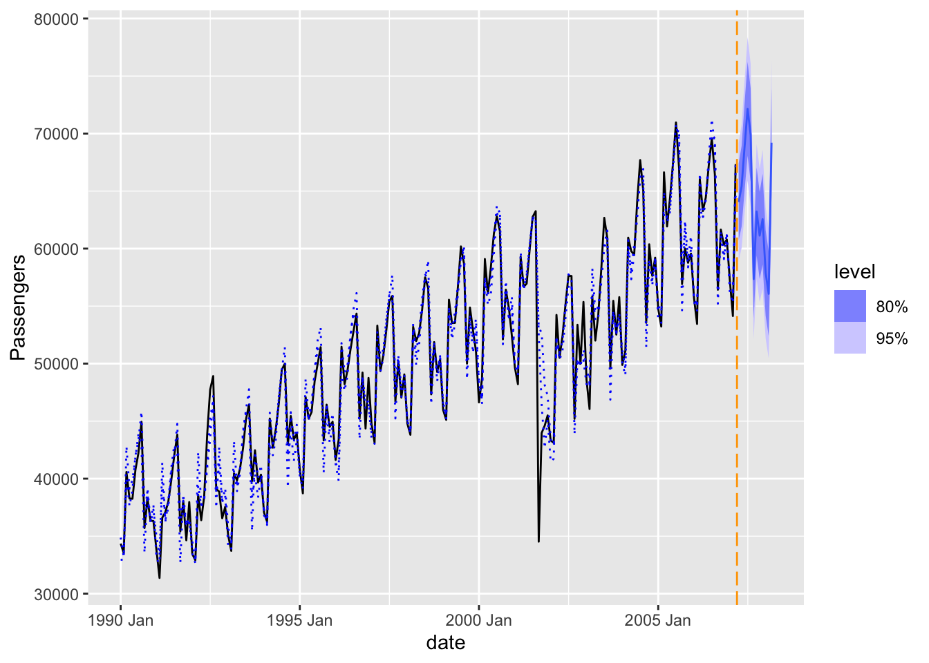
Lastly, we will plot our final model and its forecast.

Code

model_HW_for %>% 
  filter(.model=='HWM') %>%
  autoplot(train) + 
  autolayer(fitted(model_HW), col = "blue", linetype = "dotted") + 
  geom_vline(xintercept = as_date("2007-03-15"),color="orange",linetype="longdash")

Plot variable not specified, automatically selected `.vars = .fitted`

To build out our exponential smoothing models, we will need the HoltWinters function from the statsforecast.models package. For other types of exponential smoothing models, you will need different functions, such as SimpleExponentialSmoothing, SeasonalExponentialSmoothing, and Holt. In our StatsForecast function we use the model = option along with two calls of the HoltWinters function to build two models - a multiplicative Holt Winters and an additive Holt Winters. For both of these models we specify the season length of 12 observations. The main difference is the error_type = option. For multiplicative seasonal models we have "M" and for additive seasonal models we have "A". The alias option is used to define names for our models to signify which output we are seeing. From there we specify the freq = 'ME' option since we are providing the function with monthly data. Lastly, we just use the .fit function on this model with the training dataset as our input (df = train_sf).

To see how well our models performed, we need to look at different summaries of the model. To see what things that StatsForecast provides we print the .fitted_[0,0].model_.keys() function. From this output we see we can print out metrics like AIC, AICc, and BIC. We save the individual models indexed by 0 for the multiplicative Holt Winters and 1 for the additive Holt Winters in two separate model results objects. From there we print out the AIC, AICc, and BIC values for comparison.

Code

from statsforecast.models import HoltWinters

model_HW = StatsForecast(models = [HoltWinters(season_length = 12, error_type="M", alias = "HWM"), HoltWinters(season_length = 12, error_type="A", alias = "HWA")], freq = 'ME')
model_HW.fit(df = train_sf)

StatsForecast(models=[HWM,HWA])

Code

print(model_HW.fitted_[0,0].model_.keys())

dict_keys(['loglik', 'aic', 'bic', 'aicc', 'mse', 'amse', 'fit', 'residuals', 'components', 'm', 'nstate', 'fitted', 'states', 'par', 'sigma2', 'n_params', 'method', 'actual_residuals'])

Code

result_HWM = model_HW.fitted_[0,0].model_
print("Mult. AIC =", result_HWM['aic'], "\nMult. AICc =", result_HWM['aicc'], "\nMult. BIC =", result_HWM['bic'])

Mult. AIC = 4318.982810183868 
Mult. AICc = 4322.220905421964 
Mult. BIC = 4375.63902966938

Code

result_HWA = model_HW.fitted_[0,1].model_
print("Add. AIC =", result_HWA['aic'], "\nAdd. AICc =", result_HWA['aicc'], "\nAdd. BIC =", result_HWA['bic'])

Add. AIC = 4280.126926196715 
Add. AICc = 4283.765224069056 
Add. BIC = 4340.115864475492

All of these metrics point to the additive Holt Winters model being a better fit for our data than the multiplicative model. However, let’s forecast the next 12 observations (h = 12) using the .forecast function on both of our models to see how well they do on the test dataset. We also need to give the function the training data and tell it what confidence level we would like to build around our forecasts. We then use the .plot function to plot both forecasts out.

Code

model_HW_for = model_HW.forecast(df = train_sf, h = 12, level = [95])

model_HW.plot(train_sf, model_HW_for)

Let’s see how well each forecast does on our training dataset by calculated the mean absolute percentage error (MAPE) which we calculate below.

Code

error = np.array(test['Passengers']) - np.array(model_HW_for['HWM'])
MAPE = np.mean(abs(error)/test['Passengers'])*100
print("Mult. MAE =", np.mean(abs(error)), "\nMult. MAPE =", MAPE)

Mult. MAE = 802.1165364583334 
Mult. MAPE = 1.2450151759471577

Code

error = np.array(test['Passengers']) - np.array(model_HW_for['HWA'])
MAPE = np.mean(abs(error)/test['Passengers'])*100
print("Add. MAE =", np.mean(abs(error)), "\nAdd. MAPE =", MAPE)

Add. MAE = 1839.9680989583333 
Add. MAPE = 2.850081334857867

To build out our exponential smoothing models, we will use the PROC ESM procedure. In the PROC ESM statement we specify the training dataset with the data = option. We will only have it print out the model fit statistics (print = statistics) and plot the forecasts (plot = forecasts). We tell SAS that the length of our season is 12 observations with the seasonality = 12 option and ask it to forecast 12 observations with the lead = 12 option. Lastly, we ask it to save our forecasts as a new dataset with the outfor = option. Next, in the FORECAST statement we specify our target variable, Passengers, and the model as the additive Holt Winters model (model = addwinters). We will run another PROC ESM with the exact same options except for the model which will be the multiplicative Holt Winters model (model = winters).

Code

proc esm data = work.train print = statistics plot = forecasts seasonality = 12 lead = 12 outfor = work.HWAfor;
    forecast Passengers / model = addwinters;
run;

proc esm data = work.train print = statistics plot = forecasts seasonality = 12 lead = 12 outfor = work.HWMfor;
    forecast Passengers / model = winters;
run;

The first table of output corresponds to the additive Holt Winters model, while the second corresponds to the multiplicative Holt Winters model. There are a large number of metrics that we can look at to compare these models. From the AIC, SBC, MAE, and MAPE values it appears that the multiplicative Holt Winters is slightly better than the additive version. However, since they are so close we will look at both of them compared to the test dataset.

First, we need to isolate just the forecasted observations from the output above. For that we use the DATA STEP to just look at the predicted values from the two previous models beyond the 207 training observations with the WHERE statement. Next, we use the MERGE statement in another DATA STEP to merge the original test dataset with the predicted values from both of the models. Lastly, we calculate the absolute error and absolute percentage error for each observation with our last DATA STEP. To get the average of these calculations, we throw our test dataset into the PROC MEANS procedure where we specify these variables with the VAR statement.

Code

data HWAFOR;
    set HWAFOR;
    where _timeid_ > 207;
    Predict_HWA = Predict;
    keep Predict_HWA;
run;

data HWMFOR;
    set HWMFOR;
    where _timeid_ > 207;
    Predict_HWM = Predict;
    keep Predict_HWM;
run;

data test;
    merge test HWAFOR HWMFOR;
run;

data test;
    set test;
    AE_HWM = abs(Passengers - Predict_HWM);
    AE_HWA = abs(Passengers - Predict_HWA);
    APE_HWM = abs(Passengers - Predict_HWM)/Passengers*100;
    APE_HWA = abs(Passengers - Predict_HWA)/Passengers*100;
run;

proc means data = test;
    var AE_HWM APE_HWM AE_HWA APE_HWA;
run;

Lastly, we will show the plot of our final model and its forecast that we originally got from the PROC ESM output.

--- title: "Exponential Smoothing Models" format: html: code-fold: show code-tools: true editor: visual --- ```{r} #| include: false #| warning: false #| message: false library(fpp3) file.dir = "https://raw.githubusercontent.com/sjsimmo2/TimeSeries/master/" input.file1 = "usairlines.csv" USAirlines = read.csv(paste(file.dir, input.file1,sep = "")) USAirlines <- USAirlines %>% mutate(date = yearmonth(lubridate::make_date(Year, Month))) USAirlines_ts <- as_tsibble(USAirlines, index = date) train <- USAirlines_ts %>% select(Passengers, date, Month) %>% filter_index(~ "2007-03") test <- USAirlines_ts %>% select(Passengers, date, Month) %>% filter_index("2007-04" ~ .) ``` ```{python} #| include: false #| warning: false #| message: false import pandas as pd import numpy as np import matplotlib.pyplot as plt import statsmodels.api as sm import seaborn as sns from statsforecast import StatsForecast usair = pd.read_csv("https://raw.githubusercontent.com/sjsimmo2/TimeSeries/master/usairlines.csv") df = pd.date_range(start = '1/1/1990', end = '3/1/2008', freq = 'MS') usair.index = pd.to_datetime(df) train = usair.head(207) test = usair.tail(12) d = {'unique_id': 1, 'ds': train.index, 'y': train['Passengers']} train_sf = pd.DataFrame(data = d) d = {'unique_id': 1, 'ds': test.index, 'y': test['Passengers']} test_sf = pd.DataFrame(data = d) ``` # Quick Summary {{< video https://www.youtube.com/embed/hAD5vVz07ZA?si=GuqJuNM521bKF74B >}} # Time Dependency Time series data relies on the assumption that the observations at a certain time point depend on previous observations in time. The most extreme versions of this assumption is the **naive model** and the **average model**. The naive model assumes that any prediction in the future (*h* observations) is just the latest known value at the current time, *t:* $$ \hat{Y}_{t+h} = Y_t $$ The average model is the other extreme that assumes that any prediction in the future (*h* observations) are the equally weighted average of all of the data in the past: $$ \hat{Y}_{t+h} = \frac{1}{T} \sum^T_{t=1} Y_t $$ Obviously, a better approach might be to use all of the data (like the average model) but emphasize more recent data (like the naive model) more heavily. The is the approach of the class of models called **exponential smoothing models (ESMs)**. In exponential smoothing models the weights on the observations emphasize the most recent data, requires only estimating a few parameters, and are simple and easy to implement. There are many different types of exponential smoothing models. Here we will discuss three common types: 1. Single (or Simple) ESM 2. Linear / Holt (incorporating trend) ESM 3. Holt-Winters (incorporating trend and seasonality) ESM # Single Exponential Smoothing In single exponential smoothing we apply a weighting scheme that decreases exponentially the further back in time we go: $$ \hat{Y}_{t+1} = \theta Y_t + \theta (1 - \theta) Y_{t-1} + \theta (1 - \theta)^2 Y_{t-2} + \theta(1 - \theta)^3 Y_{t-3} + \cdots $$ where $0 \le \theta \le 1$. The previous equation for the single exponential smoothing model can be written more simply as the following: $$ \hat{Y}_{t+1} = \theta Y_t + (1 - \theta)Y_t $$ The single exponential smoothing model can also be written in **component form**: $$ \hat{Y}_{t+1} = L_t $$ $$ L_t = \theta Y_t + (1 - \theta)L_{t-1} $$ where the first equation is the forecast equation and the second equation is the level equation. The larger the value of $\theta$, the more that the most recent observation is emphasized as shown by the chart below.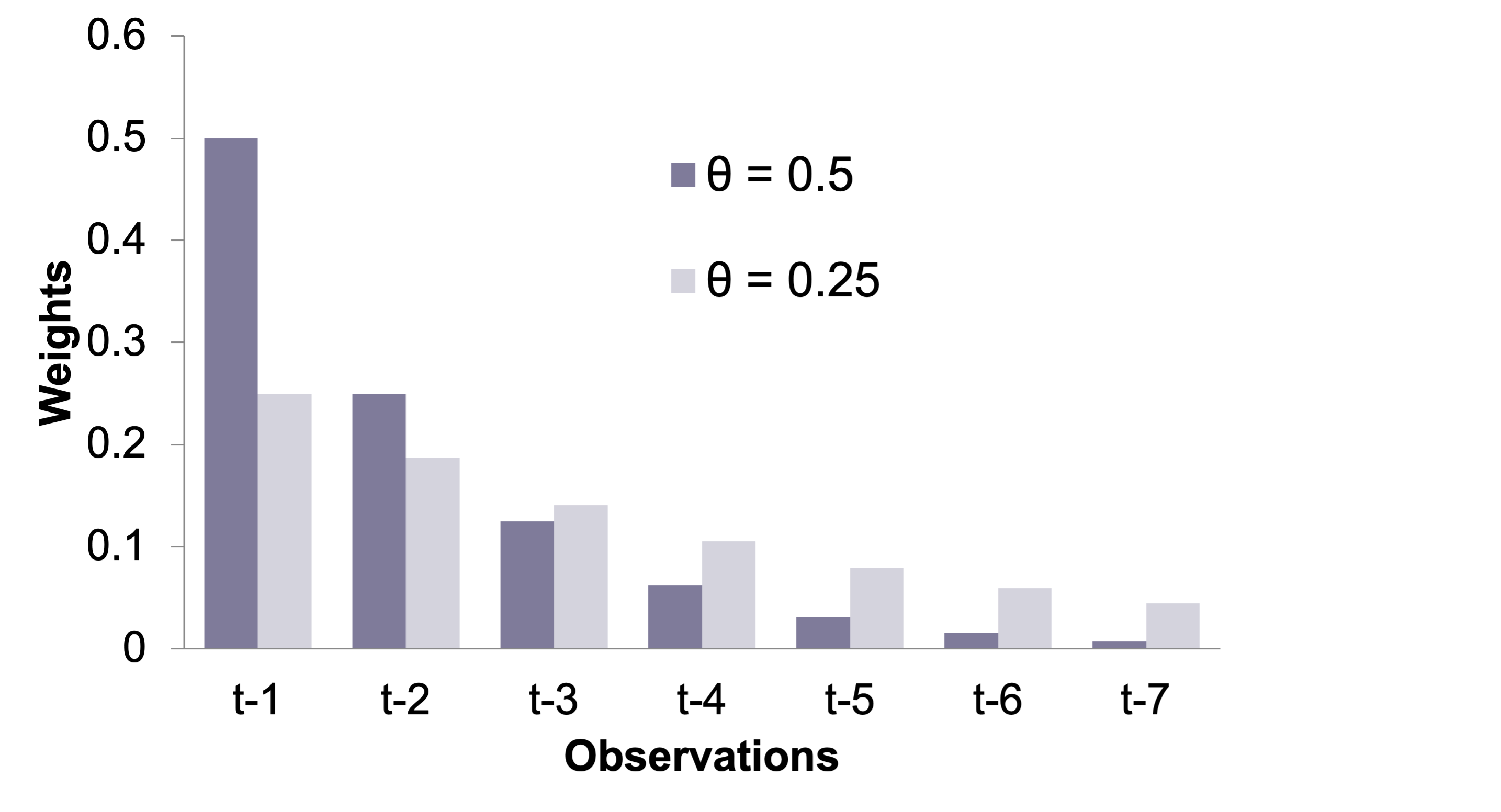 ![](image/Theta.png){fig-align="center" width="5.52in"} The optimal value of $\theta$ is the value that minimizes the one-step ahead forecast errors using the sum of these squared errors: $$ SSE = \sum_{t=1}^T (Y_t - \hat{Y}_t)^2 $$ Visually, this looks like the following picture: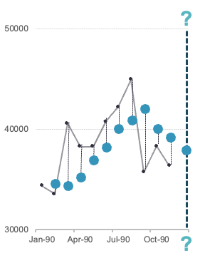 ![](image/SSE.png){fig-align="center" width="3.06in"} where each of the dashed lines in the plot above would be squared and summed together. That value of $\theta$ that minimizes that quantity is the optimal value. The only downside of optimizing only for the next time period is that you only get a forecast that is one value in the future. Any forecast beyond the initial point is the exact same as the initially forecasted point. Some statistical software will report statistical tests for the $\theta$ parameter, but not everyone considers the results of these tests because the model was never derived and designed with statistical distributions and significance in mind. # Trending Exponential Smoothing The single exponential smoothing model is better used for short-term forecasts. That model cannot adequately handle data that is trending up or down. There are multiple ways to incorporate a trend component in the exponential smoothing framework. - Brown / Double exponential smoothing - Holt / Linear exponential smoothing - Damped Trend exponential smoothing ## Brown Exponential Smoothing The double / Brown exponential smoothing model has two components - level and trend. The trend component incorporates an exponential smoothing calculation on the trend component: $$ \hat{Y}_{t+k} = L_t + k T_t $$ $$ L_t = \theta Y_t + (1 - \theta)(L_{t-1} + T_{t-1}) $$ $$ T_t = \theta(L_t - L_{t-1}) + (1 - \theta)T_{t-1} $$ where the value of $k$ is the number of observations to be forecasted. The only problem with the Brown exponential smoothing model is the unrealistic assumption that the $\theta$ in the level component is the same as the $\theta$ in the trend component. ## Holt Exponential Smoothing The Holt exponential smoothing model also has two components - level and trend. The only difference between this model and the Brown exponential smoothing model is that there are different parameters for the level and trend components: $$ \hat{Y}_{t+k} = L_t + k T_t $$ $$ L_t = \theta Y_t + (1 - \theta)(L_{t-1} + T_{t-1}) $$ $$ T_t = \gamma(L_t - L_{t-1}) + (1 - \gamma)T_{t-1} $$ where the value of $k$ is the number of observations to be forecasted. The optimal values of $\theta$ and $\gamma$ are determined by minimizing the sum of squared errors where the trend component is calculated with the one-step ahead forecast error as seen below: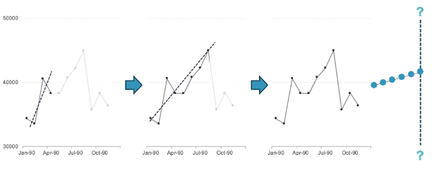 ![](image/TrendESM.png){fig-align="center" width="10.11in"} Similar to the single exponential smoothing model, the Holt exponential smoothing model is optimized to predict the next forecasted value. However, unlike the single exponential smoothing model, this model follows the trend line after that first predicted value. ## Damped Trend Exponential Smoothing The Holt exponential smoothing model also has two components - level and trend. The only difference between this model and the Holt exponential smoothing model is that the trend component isn't just added on to the level component. Instead the trend component is dampened as the forecast horizon gets larger: $$ \hat{Y}_{t+k} = L_t + \sum_{i=1}^k \phi^i T_t $$ $$ L_t = \theta Y_t + (1 - \theta)(L_{t-1} + \phi T_{t-1}) $$ $$ T_t = \gamma(L_t - L_{t-1}) + (1 - \gamma)\phi T_{t-1} $$ where the value of $k$ is the number of observations to be forecasted and $0 \le \phi \le 1$. The optimal values of $\theta$, $\phi$, and $\gamma$ are determined by minimizing the sum of squared errors where the trend component is calculated with the one-step ahead forecast error. # Seasonal Exponential Smoothing Exponential smoothing models can also account for seasonal factors. In seasonal exponential smoothing models, weights decay with respect to the seasonal factor: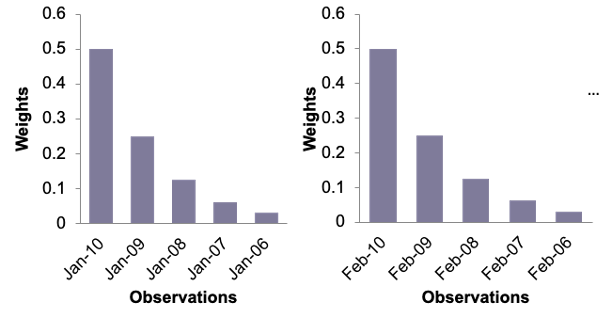 ![](image/SeasESM.png){fig-align="center" width="5.78in"} There are multiple ways to incorporate a seasonal effect in the exponential smoothing framework. - Winters Additive Seasonal ESM - Winters Multiplicative Seasonal ESM - Holt Winters Additive Seasonal ESM - Holt Winters Multiplicative Seasonal ESM ## Winters Seasonal Exponential Smoothing If your data is seasonal in structure, but has no trend, then the Winters seasonal exponential smoothing model is a good model to use. Instead of the trend component that we saw in the Holt exponential smoothing model, the Winters model includes a seasonal component. Similar to what we saw with time series decomposition, the seasonal term can have an additive or multiplicative structure: Additive Seasonal Component: $$ \hat{Y}_{t+k} = L_t + S_{t-p+k} $$ $$ L_t = \theta (Y_t - S_{t-p}) + (1 - \theta)L_{t-1} $$ $$ S_t = \delta(Y_t - L_t) + (1 - \delta)S_{t-p} $$ Multiplicative Seasonal Component: $$ \hat{Y}_{t+k} = L_t \times S_{t-p+k} $$ $$ L_t = \theta (Y_t / S_{t-p}) + (1 - \theta)L_{t-1} $$ $$ S_t = \delta(Y_t / L_t) + (1 - \delta)S_{t-p} $$ where $k$ is the number of observations to be forecasted. From the above equations we can see that the only difference is that we either add in the seasonal component, or multiply in the seasonal component. The optimal values of $\theta$ and $\delta$ are determined by minimizing the sum of squared errors of the one-step ahead forecast error. However, with the seasonal component, one-step ahead is one season ahead which means the model is optimized to predict one season into the future, instead of just one observation.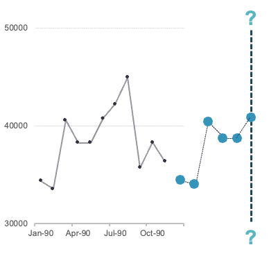 ![](image/WinterPred.png){fig-align="center" width="4.12in"} ## Holt Winters Seasonal Exponential Smoothing If your data is seasonal in structure, and has a trend, then the Holt Winters (Triple) seasonal exponential smoothing model is a good model to use. Instead addition to the trend component that we saw in the Holt exponential smoothing model, the Holt Winters model includes a seasonal component as well. Similar to what we saw with time series decomposition, the seasonal term can have an additive or multiplicative structure: Additive Seasonal Component: $$ \hat{Y}_{t+k} = L_t + k T_t + S_{t-p+k} $$ $$ L_t = \theta (Y_t - S_{t-p}) + (1 - \theta)(L_{t-1} + T_{t-1}) $$ $$ T_t = \gamma(L_t - L_{t-1}) + (1 - \gamma) T_{t-1} $$ $$ S_t = \delta(Y_t - L_t) + (1 - \delta)S_{t-p} $$ Multiplicative Seasonal Component: $$ \hat{Y}_{t+k} = (L_t + k T_t) \times S_{t-p+k} $$ $$ L_t = \theta (Y_t / S_{t-p}) + (1 - \theta)(L_{t-1} + T_{t-1}) $$ $$ T_t = \gamma(L_t - L_{t-1}) + (1 - \gamma) T_{t-1} $$ $$ S_t = \delta(Y_t / L_t) + (1 - \delta)S_{t-p} $$ where $k$ is the number of observations to be forecasted. From the above equations we can see that the only difference is that we either add in the seasonal component, or multiply in the seasonal component. The optimal values of $\theta$, $\gamma$, and $\delta$ are determined by minimizing the sum of squared errors of the one-step ahead forecast error. However, with the seasonal component, one-step ahead is one season ahead which means the model is optimized to predict one season into the future along a trend line, instead of just one observation.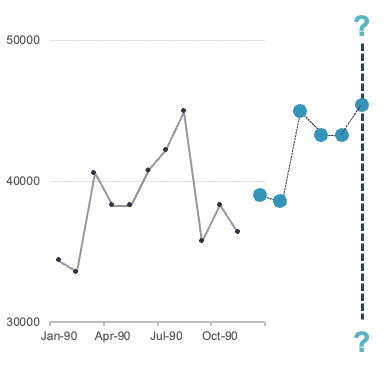 ![](image/HWPred.png){fig-align="center" width="4.12in"} Since our data has both a trend and seasonal component, we will build a Holt Winters Exponential smoothing model. Let's see how to do that in all of our software! ::: {.panel-tabset .nav-pills} ## R To build out our exponential smoothing models, we will still use the `model` function on our training dataset. The `model` function can specify multiple models to build at once for comparing against each other. To build an exponential smoothing model we use the `ETS` function in the `model` function. Within the `ETS` function we write a formula specifying the model we want. Here we have our target variable, *Passengers*, on the left hand side of the `~` followed by our components from the ESM's. For the first model (which we name *HWM*, we will build a multiplicative Holt Winters model. For the multiplicative Holt Winters we specify the additive trend term (`trend("A")`), and the multiplicative seasonal term (`season("M")` and `error("M")`). Although the error and season don't have to match, that would be a different structure than the Holt Winters model. The same thing can be done with our second model named *HWA*. We use the `ETS` function still, but instead we put in an additive season and error component to get the additive Holt Winters model. It is easy to see how you could get other exponential smoothing models we have discussed by removing different components from the formula. From there we will use the `glance` function to look at some basic summaries about each model to compare how well they did with our training data. We then use the `forecast` function from the `fabletools` package to forecast out 12 observations (`h = 12`) in the future. We then finish up with the `autoplot` function to plot the forecasts from each of our models. ```{r} model_HW <- train %>% model( HWM = ETS(Passengers ~ error("M") + trend("A") + season("M")), HWA = ETS(Passengers ~ error("A") + trend("A") + season("A")) ) glance(model_HW) model_HW_for <- model_HW %>% fabletools::forecast(h = 12) model_HW_for %>% autoplot(train) ``` Let's compare the above models. Its seems like they are extremely close in terms of their performance on the training dataset. The log-likelihood, AIC, AICc, and BIC values are all nearly identical. Even the plot looks like they have very similar predictions. In this scenario, we will take both model to the test dataset to see which performs better. For that we will use the `accuracy` function from the `fabletools` package. The inputs to this function are our model object and the test dataset. ```{r} fabletools::accuracy(model_HW_for, test) ``` From the output above, it seems like the multiplicative Holt Winters model beats out the additive version on the test dataset on the metrics of mean absolute error (MAE) and mean absolute percentage error (MAPE). This will be our model and metric to try and beat for the rest of the techniques that we learn. The exponential smoothing model is a wonderful, first model to build with any time series dataset. You will be surprised at how hard it is to beat one of these models, especially if you are only forecasting in the short term. Here, we are only forecasting a single year, which the Holt Winters exponential smoothing model is optimized to do given the yearly seasonality of our data. Lastly, we will plot our final model and its forecast. ```{r} model_HW_for %>% filter(.model=='HWM') %>% autoplot(train) + autolayer(fitted(model_HW), col = "blue", linetype = "dotted") + geom_vline(xintercept = as_date("2007-03-15"),color="orange",linetype="longdash") ``` ## Python To build out our exponential smoothing models, we will need the `HoltWinters` function from the `statsforecast.models` package. For other types of exponential smoothing models, you will need different functions, such as `SimpleExponentialSmoothing`, `SeasonalExponentialSmoothing`, and `Holt`. In our `StatsForecast` function we use the `model =` option along with two calls of the `HoltWinters` function to build two models - a multiplicative Holt Winters and an additive Holt Winters. For both of these models we specify the season length of 12 observations. The main difference is the `error_type =` option. For multiplicative seasonal models we have `"M"` and for additive seasonal models we have `"A"`. The `alias` option is used to define names for our models to signify which output we are seeing. From there we specify the `freq = 'ME'` option since we are providing the function with monthly data. Lastly, we just use the `.fit` function on this model with the training dataset as our input (`df = train_sf`). To see how well our models performed, we need to look at different summaries of the model. To see what things that `StatsForecast` provides we print the `.fitted_[0,0].model_.keys()` function. From this output we see we can print out metrics like AIC, AICc, and BIC. We save the individual models indexed by 0 for the multiplicative Holt Winters and 1 for the additive Holt Winters in two separate model results objects. From there we print out the AIC, AICc, and BIC values for comparison. ```{python} from statsforecast.models import HoltWinters model_HW = StatsForecast(models = [HoltWinters(season_length = 12, error_type="M", alias = "HWM"), HoltWinters(season_length = 12, error_type="A", alias = "HWA")], freq = 'ME') model_HW.fit(df = train_sf) print(model_HW.fitted_[0,0].model_.keys()) result_HWM = model_HW.fitted_[0,0].model_ print("Mult. AIC =", result_HWM['aic'], "\nMult. AICc =", result_HWM['aicc'], "\nMult. BIC =", result_HWM['bic']) result_HWA = model_HW.fitted_[0,1].model_ print("Add. AIC =", result_HWA['aic'], "\nAdd. AICc =", result_HWA['aicc'], "\nAdd. BIC =", result_HWA['bic']) ``` All of these metrics point to the additive Holt Winters model being a better fit for our data than the multiplicative model. However, let's forecast the next 12 observations (`h = 12`) using the `.forecast` function on both of our models to see how well they do on the test dataset. We also need to give the function the training data and tell it what confidence level we would like to build around our forecasts. We then use the `.plot` function to plot both forecasts out. ```{python} #| warning: false #| message: false model_HW_for = model_HW.forecast(df = train_sf, h = 12, level = [95]) model_HW.plot(train_sf, model_HW_for)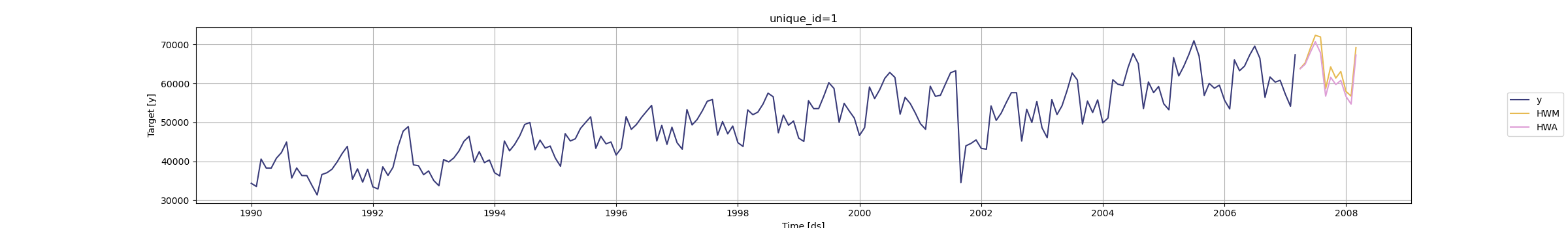 ``` ![](image/plot_for_HW.png){fig-align="center" width="34.31in"} Let's see how well each forecast does on our training dataset by calculated the mean absolute percentage error (MAPE) which we calculate below. ```{python} error = np.array(test['Passengers']) - np.array(model_HW_for['HWM']) MAPE = np.mean(abs(error)/test['Passengers'])*100 print("Mult. MAE =", np.mean(abs(error)), "\nMult. MAPE =", MAPE) error = np.array(test['Passengers']) - np.array(model_HW_for['HWA']) MAPE = np.mean(abs(error)/test['Passengers'])*100 print("Add. MAE =", np.mean(abs(error)), "\nAdd. MAPE =", MAPE) ``` From the output above, it seems like the multiplicative Holt Winters model beats out the additive version on the test dataset on the metrics of mean absolute error (MAE) and mean absolute percentage error (MAPE). This will be our model and metric to try and beat for the rest of the techniques that we learn. The exponential smoothing model is a wonderful, first model to build with any time series dataset. You will be surprised at how hard it is to beat one of these models, especially if you are only forecasting in the short term. Here, we are only forecasting a single year, which the Holt Winters exponential smoothing model is optimized to do given the yearly seasonality of our data. ## SAS To build out our exponential smoothing models, we will use the PROC ESM procedure. In the PROC ESM statement we specify the training dataset with the `data =` option. We will only have it print out the model fit statistics (`print = statistics`) and plot the forecasts (`plot = forecasts`). We tell SAS that the length of our season is 12 observations with the `seasonality = 12` option and ask it to forecast 12 observations with the `lead = 12` option. Lastly, we ask it to save our forecasts as a new dataset with the `outfor =` option. Next, in the FORECAST statement we specify our target variable, *Passengers*, and the model as the additive Holt Winters model (`model = addwinters`). We will run another PROC ESM with the exact same options except for the model which will be the multiplicative Holt Winters model (`model = winters`). ```{r} #| eval: false proc esm data = work.train print = statistics plot = forecasts seasonality = 12 lead = 12 outfor = work.HWAfor; forecast Passengers / model = addwinters; run; proc esm data = work.train print = statistics plot = forecasts seasonality = 12 lead = 12 outfor = work.HWMfor; forecast Passengers / model = winters; run;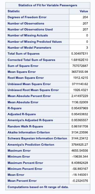 ``` ![](image/3_a_SAS.png){fig-align="center" width="3.15in"}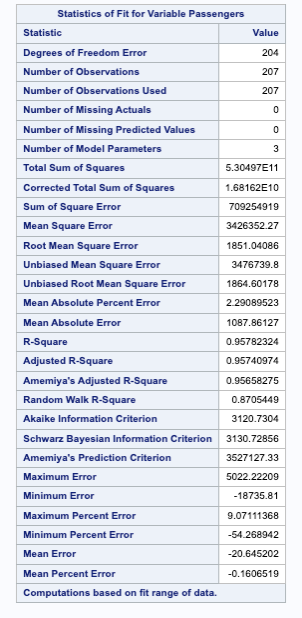 ![](image/3_b_SAS.png){fig-align="center" width="3.15in"} The first table of output corresponds to the additive Holt Winters model, while the second corresponds to the multiplicative Holt Winters model. There are a large number of metrics that we can look at to compare these models. From the AIC, SBC, MAE, and MAPE values it appears that the multiplicative Holt Winters is slightly better than the additive version. However, since they are so close we will look at both of them compared to the test dataset. First, we need to isolate just the forecasted observations from the output above. For that we use the DATA STEP to just look at the predicted values from the two previous models beyond the 207 training observations with the WHERE statement. Next, we use the MERGE statement in another DATA STEP to merge the original test dataset with the predicted values from both of the models. Lastly, we calculate the absolute error and absolute percentage error for each observation with our last DATA STEP. To get the average of these calculations, we throw our test dataset into the PROC MEANS procedure where we specify these variables with the VAR statement. ```{r} #| eval: false data HWAFOR; set HWAFOR; where _timeid_ > 207; Predict_HWA = Predict; keep Predict_HWA; run; data HWMFOR; set HWMFOR; where _timeid_ > 207; Predict_HWM = Predict; keep Predict_HWM; run; data test; merge test HWAFOR HWMFOR; run; data test; set test; AE_HWM = abs(Passengers - Predict_HWM); AE_HWA = abs(Passengers - Predict_HWA); APE_HWM = abs(Passengers - Predict_HWM)/Passengers*100; APE_HWA = abs(Passengers - Predict_HWA)/Passengers*100; run; proc means data = test; var AE_HWM APE_HWM AE_HWA APE_HWA; run;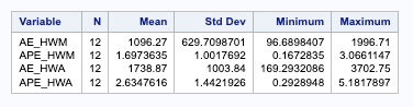 ``` ![](image/3_c_SAS.png){fig-align="center" width="5.76in"} From the output above, it seems like the multiplicative Holt Winters model beats out the additive version on the test dataset on the metrics of mean absolute error (MAE) and mean absolute percentage error (MAPE). This will be our model and metric to try and beat for the rest of the techniques that we learn. The exponential smoothing model is a wonderful, first model to build with any time series dataset. You will be surprised at how hard it is to beat one of these models, especially if you are only forecasting in the short term. Here, we are only forecasting a single year, which the Holt Winters exponential smoothing model is optimized to do given the yearly seasonality of our data. Lastly, we will show the plot of our final model and its forecast that we originally got from the PROC ESM output. ![](image/3_d_SAS.png){fig-align="center" width="5.33in"} :::