A time series is analyzed with an assumption that observations have a potential relationship that exists across periods of time. In a lot of statistical time series modeling, we try to explain this dependency using previous signals (lags) across time.
If we are successful in removing all signals we are left with independent errors, sometimes called white noise. A white noise process (or time series itself) follows a Normal (Gaussian) distribution with a mean of zero and positive, constant variance in which all observations are independent of each other. Essentially we removed all to the correlation over time with our modeling of the signal. In other words, the autocorrelation and partial autocorrelation functions have a value of 0 at every point lag (except for lag 0).
Unlike exponential smoothing models where the goal was minimizing the one-step ahead forecast error and focus solely on predictive power, the goal of a lot of statistical time series modeling (like autoregressive or moving average models) is to be left with white noise residuals. If the residuals have a correlation structure still, then more modeling might be able to be done.
It would not be surprising that the autocorrelation and partial autocorrelation functions on the residuals are not perfectly 0 because of sample variability. The Ljung-Box \(\chi^2\) test statistically tests for white noise.
The value of \(\hat{\rho}_k\) in the above equation is the autocorrelation function at lag k. The null hypothesis is white noise while the alternative hypothesis of this test is at least one of the lags is not 0. If the autocorrelations are all close to zero, then the test statistic is low which would make the p-value high. If any of the autocorrelations are not close to zero (up to whatever lag m you are testing) then the test statistic would be high leading to small p-value.
Let’s see how to calculate this in each of our softwares!
Although the exponential smoothing model’s goal is to be predictive in the short term and not necessarily remove all of the signal out of the data, we will still use it as our example. Let’s examine the residuals of our exponential smoothing model and test if they are white noise.
We built the ESM with the same process we had in the section on exponential smoothing. Here we have our Holt-Winters exponential smoothing model with a multiplicative seasonal effect. We can use the augment function to calculate things on the output from this model. With the features function we can look at the ljung_box option up to a lag of 36. We are using three degrees of freedom (dof = 3) because of the number of parameters that needed to be estimated in the Holt-Winters ESM.
For our sample size a significance level, \(\alpha\), of 0.02 would be reasonable. At this significance level our residuals from the Holt-Winters ESM is not white noise because we rejected the null hypothesis of white noise due to this low p-value.
Although the exponential smoothing model’s goal is to be predictive in the short term and not necessarily remove all of the signal out of the data, we will still use it as our example. Let’s examine the residuals of our exponential smoothing model and test if they are white noise.
We built the ESM with the same process we had in the section on exponential smoothing. Here we have our Holt-Winters exponential smoothing model with a multiplicative seasonal effect. We can use the acorr_ljungbox function from the statsmodels package to calculate things on the output from this model. With the lag = option we can look up to a lag of 36. We are using three degrees of freedom (model_df = 3) because of the number of parameters that needed to be estimated in the Holt-Winters ESM.
For our sample size a significance level, \(\alpha\), of 0.02 would be reasonable. At this significance level our residuals from the Holt-Winters ESM is not white noise because we rejected the null hypothesis of white noise due to this low p-value.
Although the exponential smoothing model’s goal is to be predictive in the short term and not necessarily remove all of the signal out of the data, we will still use it as our example. Let’s examine the residuals of our exponential smoothing model and test if they are white noise.
We built the ESM with the same process we had in the section on exponential smoothing. Here we have our Holt-Winters exponential smoothing model with a multiplicative seasonal effect. To calculate the residuals from this model we need the outfor = option. We can use the PROC ARIMA procedure to calculate things on the output from this model. With the IDENTIFY statement we will analyze the residuals (error variable) from the output from out previous model. With the nlag = 36 option we can look up to a lag of 36. We have to “fool” SAS into modeling the data with the ARIMA PROCEDURE to get our Ljung-Box output. We use the ESTIMATE statement with no modeling parameters to do this. The method = ML option tells SAS to use maximum likelihood to calculate the model.
Code
proc esm data = work.train print = statistics seasonality =12 lead =12 outfor = work.HWMfor; forecast Passengers / model = winters;run;proc arima data = work.HWMfor plot(unpack) = all; identify var = error nlag =36; estimate method = ML;run;
For our sample size a significance level, \(\alpha\), of 0.02 would be reasonable. At this significance level our residuals from the Holt-Winters ESM is white noise because we cannot reject the null hypothesis of white noise due to this higher p-value from the table above. The plot above is a little hard to grasp at first. The bars more represent the test statistics than the p-values. Larger test statistics would lead to smaller p-values. The alpha levels are marked on the y-axis to show you if the test statistic is too large.
Stationarity
In time series we assume that there exists a dependence structure to our time series data. Even though we do not want independent observations, some modeling techniques want some consistency in our time series to make the modeling possible. The group of models called stationary models want the data to be stationary (or have stationarity).
Stationarity is where the distribution of the data depends only on the difference in time, not on the location in time. For example, we want a consistent mean, variance, and autocorrelation. In other words, the mean, variance, and autocorrelation of our data should not depend on where in the time series we are, but how big the window of time we are looking at. This automatically implies that data with long-term trend or seasonal components can not be stationary because the mean of the series depends on the time that the values are observed.
This is probably best seen with an example. Let’s look back at the naive model introduced in the section on exponential smoothing:
\[
Y_t = Y_{t-1} + e_t
\]
where your guess of today is just what the value was yesterday knowing there is some error around that. This model is also called the random walk model. If your model is drifting one way or another, the random walk model can turn into the random walk with drift model:
\[
Y_t = \omega + Y_{t-1} + e_t
\]
The autocorrelation and partial autocorrelation functions for the random walk model are in the plots below.
We can see in the PACF plot above that the impact felt in the current time is only coming directly from the previous time point and none before that. However, in the ACF we see that persistence across all time because the current time is impacted by the previous one, the previous one impacted by the one before that and so on. Therefore, the impact of any time point in a random walk is felt forever and continues across all of time. That means that every data point has full impact no matter how long ago it was. This makes forecasting a random walk practically impossible. Although we assume a dependence structure to our time series, we also want this dependence to decrease over time. We don’t want an observation to influence our data forever.
This complete persistence of past data another sign of non-stationary data. Although a stationary time series can be short, medium, or long-term memory, the impacts of observations must decrease with time. All stationary models mathematically revert to the mean of the data series in their forecasts. The long-term memory model still generates models that revert to the mean, just much slower than a short-term memory model.
Non-Stationarity
Non-stationarity in data can occur when your data dependencies don’t dissipate as time goes on, you have a trend, or you have a seasonal component to your data. Does this mean we cannot use stationary modeling techniques to model non-stationary data? No, but we have to make our data stationary before we can use stationary modeling techniques like AR, MA, or ARIMA modeling.
There are two schools of thought around how to handle non-stationary data.
Stationarity Testing
There are many formal statistical tests for testing the stationarity of time series data. One of the most widely used is the Augmented Dickey-Fuller (ADF) test. There are 3 different forms to this test:
Zero Mean
Single Mean
Trend
If your data has no seasonality and no trend, then either of the first two tests are the ones to use depending on whether your data has an average of 0 (the zero mean test) or an average other then 0 (the single mean test). If your data is trending, then you would need to use the trend test.
Let’s look at the most basic structure of each of these forms of the Dickey-Fuller test. For the zero mean test the model being tested is:
\[
Y_t = \phi Y_{t-1} + e_t
\]
with the null hypothesis of \(H_0: \phi = 1\) (non-stationary) and the alternative hypothesis of \(H_a: |\phi| < 1\) (stationary around 0).
For the single mean test the model being tested is:
\[
Y_t - \mu = \phi(Y_{t-1} - \mu) +e_t
\]
with the null hypothesis of \(H_0: \phi = 1\) (non-stationary) and the alternative hypothesis of \(H_a: |\phi| < 1\) (stationary around a mean \(\mu\)).
with the null hypothesis of \(H_0: \phi = 1\) (non-stationary) and the alternative hypothesis of \(H_a: |\phi| < 1\) (stationary around the trend line). The best part of the ADF test for trend is that not only does it tell us if our data is stationary, but how to solve the non-stationary trend in your data. With trending data, if the trend test rejects the null hypothesis then a trend line is the better solution (deterministic solution) to handle trend as compared to taking a difference (stochastic solution). These trend solutions of either fitting a trend line or taking a difference are discussed in the next section below.
Non-stationary data are not limited to random walks with only one lag. The Augmented Dickey-Fuller (ADF) test can be done on models with more lags than the ones seen above.
Let’s see how to do this in each of our softwares!
---title: "Stationarity"format: html: code-fold: show code-tools: trueeditor: visual---```{r}#| include: false#| warning: false#| message: falselibrary(fpp3)file.dir ="https://raw.githubusercontent.com/sjsimmo2/TimeSeries/master/"input.file1 ="usairlines.csv"USAirlines =read.csv(paste(file.dir, input.file1,sep =""))USAirlines <- USAirlines %>%mutate(date =yearmonth(lubridate::make_date(Year, Month)))USAirlines_ts <-as_tsibble(USAirlines, index = date)train <- USAirlines_ts %>%select(Passengers, date, Month) %>%filter_index(~"2007-03")test <- USAirlines_ts %>%select(Passengers, date, Month) %>%filter_index("2007-04"~ .)``````{python}#| include: false#| warning: false#| message: falseimport pandas as pdimport numpy as npimport matplotlib.pyplot as pltimport statsmodels.api as smimport seaborn as snsfrom statsforecast import StatsForecastusair = pd.read_csv("https://raw.githubusercontent.com/sjsimmo2/TimeSeries/master/usairlines.csv")df = pd.date_range(start ='1/1/1990', end ='3/1/2008', freq ='MS')usair.index = pd.to_datetime(df)train = usair.head(207)test = usair.tail(12)d = {'unique_id': 1, 'ds': train.index, 'y': train['Passengers']}train_sf = pd.DataFrame(data = d)d = {'unique_id': 1, 'ds': test.index, 'y': test['Passengers']}test_sf = pd.DataFrame(data = d)```# Quick Summary{{< video https://www.youtube.com/embed/aIdTGKjQWjA?si=3Iv08Hl8f4wtKIro >}}# White NoiseA time series is analyzed with an assumption that observations have a potential relationship that exists across periods of time. In a lot of statistical time series modeling, we try to explain this dependency using previous signals (lags) across time.{fig-align="center" width="6.2in"}If we are successful in removing all signals we are left with independent errors, sometimes called **white noise**. A white noise process (or time series itself) follows a Normal (Gaussian) distribution with a mean of zero and positive, constant variance in which all observations are independent of each other. Essentially we removed all to the correlation over time with our modeling of the signal. In other words, the autocorrelation and partial autocorrelation functions have a value of 0 at every point lag (except for lag 0).Unlike exponential smoothing models where the goal was minimizing the one-step ahead forecast error and focus solely on predictive power, the goal of a lot of statistical time series modeling (like autoregressive or moving average models) is to be left with white noise residuals. If the residuals have a correlation structure still, then more modeling might be able to be done.It would not be surprising that the autocorrelation and partial autocorrelation functions on the residuals are not perfectly 0 because of sample variability. The Ljung-Box $\chi^2$ test statistically tests for white noise.$$\chi^2_m = n(n+2) \sum_{n-k}^m \frac{\hat{\rho}^2_k}{n-k}$$The value of $\hat{\rho}_k$ in the above equation is the autocorrelation function at lag *k*. The null hypothesis is white noise while the alternative hypothesis of this test is **at least one** of the lags is not 0. If the autocorrelations are all close to zero, then the test statistic is low which would make the p-value high. If any of the autocorrelations are not close to zero (up to whatever lag *m* you are testing) then the test statistic would be high leading to small p-value.Let's see how to calculate this in each of our softwares!::: {.panel-tabset .nav-pills}## RAlthough the exponential smoothing model's goal is to be predictive in the short term and not necessarily remove all of the signal out of the data, we will still use it as our example. Let's examine the residuals of our exponential smoothing model and test if they are white noise.We built the ESM with the same process we had in the section on exponential smoothing. Here we have our Holt-Winters exponential smoothing model with a multiplicative seasonal effect. We can use the `augment` function to calculate things on the output from this model. With the `features` function we can look at the `ljung_box` option up to a lag of 36. We are using three degrees of freedom (`dof = 3`) because of the number of parameters that needed to be estimated in the Holt-Winters ESM.```{r}model_HW <- train %>%model( HWM =ETS(Passengers ~error("M") +trend("A") +season("M")) )augment(model_HW) %>%features(.innov, ljung_box, lag =36, dof =3)```For our sample size a significance level, $\alpha$, of 0.02 would be reasonable. At this significance level our residuals from the Holt-Winters ESM is **not** white noise because we rejected the null hypothesis of white noise due to this low p-value.## PythonAlthough the exponential smoothing model’s goal is to be predictive in the short term and not necessarily remove all of the signal out of the data, we will still use it as our example. Let’s examine the residuals of our exponential smoothing model and test if they are white noise.We built the ESM with the same process we had in the section on exponential smoothing. Here we have our Holt-Winters exponential smoothing model with a multiplicative seasonal effect. We can use the `acorr_ljungbox` function from the `statsmodels` package to calculate things on the output from this model. With the `lag =` option we can look up to a lag of 36. We are using three degrees of freedom (`model_df = 3`) because of the number of parameters that needed to be estimated in the Holt-Winters ESM.```{python}from statsforecast.models import HoltWintersmodel_HW = StatsForecast(models = [HoltWinters(season_length =12, error_type="M")], freq ='ME')model_HW.fit(df = train_sf)sm.stats.acorr_ljungbox(model_HW.fitted_[0,0].model_['residuals'], lags = [36], model_df =3)```For our sample size a significance level, $\alpha$, of 0.02 would be reasonable. At this significance level our residuals from the Holt-Winters ESM is **not** white noise because we rejected the null hypothesis of white noise due to this low p-value.## SASAlthough the exponential smoothing model’s goal is to be predictive in the short term and not necessarily remove all of the signal out of the data, we will still use it as our example. Let’s examine the residuals of our exponential smoothing model and test if they are white noise.We built the ESM with the same process we had in the section on exponential smoothing. Here we have our Holt-Winters exponential smoothing model with a multiplicative seasonal effect. To calculate the residuals from this model we need the `outfor =` option. We can use the PROC ARIMA procedure to calculate things on the output from this model. With the IDENTIFY statement we will analyze the residuals (*error* variable) from the output from out previous model. With the `nlag = 36` option we can look up to a lag of 36. We have to "fool" SAS into modeling the data with the ARIMA PROCEDURE to get our Ljung-Box output. We use the ESTIMATE statement with no modeling parameters to do this. The `method = ML` option tells SAS to use maximum likelihood to calculate the model.```{r}#| eval: falseproc esm data = work.train print = statistics seasonality =12 lead =12 outfor = work.HWMfor; forecast Passengers / model = winters;run;proc arima data = work.HWMfor plot(unpack) = all; identify var = error nlag =36; estimate method = ML;run;```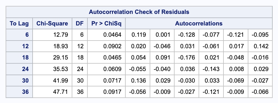{fig-align="center" width="8.09in"}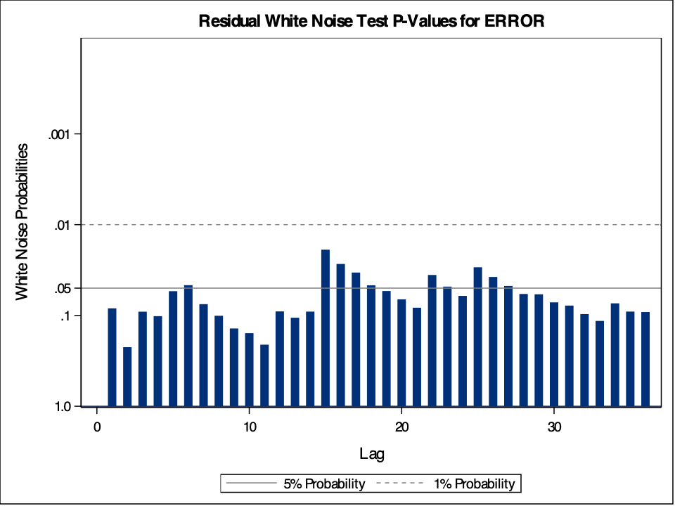{fig-align="center" width="5.33in"}For our sample size a significance level, $\alpha$, of 0.02 would be reasonable. At this significance level our residuals from the Holt-Winters ESM is white noise because we cannot reject the null hypothesis of white noise due to this higher p-value from the table above. The plot above is a little hard to grasp at first. The bars more represent the test statistics than the p-values. Larger test statistics would lead to smaller p-values. The alpha levels are marked on the y-axis to show you if the test statistic is too large.:::# StationarityIn time series we assume that there exists a dependence structure to our time series data. Even though we do not want independent observations, some modeling techniques want some consistency in our time series to make the modeling possible. The group of models called **stationary models** want the data to be stationary (or have **stationarity**).Stationarity is where the distribution of the data depends **only** on the difference in time, not on the location in time. For example, we want a consistent mean, variance, and autocorrelation. In other words, the mean, variance, and autocorrelation of our data should not depend on where in the time series we are, but how big the window of time we are looking at. This automatically implies that data with long-term trend or seasonal components can **not** be stationary because the mean of the series depends on the time that the values are observed.This is probably best seen with an example. Let's look back at the naive model introduced in the section on exponential smoothing:$$Y_t = Y_{t-1} + e_t $$where your guess of today is just what the value was yesterday knowing there is some error around that. This model is also called the **random walk model**. If your model is drifting one way or another, the random walk model can turn into the random walk with drift model:$$Y_t = \omega + Y_{t-1} + e_t$$The autocorrelation and partial autocorrelation functions for the random walk model are in the plots below.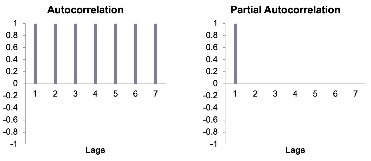{fig-align="center" width="9.2in"}We can see in the PACF plot above that the impact felt in the current time is only coming directly from the previous time point and none before that. However, in the ACF we see that persistence across all time because the current time is impacted by the previous one, the previous one impacted by the one before that and so on. Therefore, the impact of any time point in a random walk is felt forever and continues across all of time. That means that every data point has full impact no matter how long ago it was. This makes forecasting a random walk practically impossible. Although we assume a dependence structure to our time series, we also want this dependence to decrease over time. We don't want an observation to influence our data forever.This complete persistence of past data another sign of non-stationary data. Although a stationary time series can be short, medium, or long-term memory, the impacts of observations must decrease with time. All stationary models mathematically revert to the mean of the data series in their forecasts. The long-term memory model still generates models that revert to the mean, just much slower than a short-term memory model.# Non-StationarityNon-stationarity in data can occur when your data dependencies don't dissipate as time goes on, you have a trend, or you have a seasonal component to your data. Does this mean we cannot use stationary modeling techniques to model non-stationary data? No, but we have to make our data stationary before we can use stationary modeling techniques like AR, MA, or ARIMA modeling.There are two schools of thought around how to handle non-stationary data.## Stationarity TestingThere are many formal statistical tests for testing the stationarity of time series data. One of the most widely used is the Augmented Dickey-Fuller (ADF) test. There are 3 different forms to this test:1. Zero Mean2. Single Mean3. TrendIf your data has no seasonality and no trend, then either of the first two tests are the ones to use depending on whether your data has an average of 0 (the zero mean test) or an average other then 0 (the single mean test). If your data is trending, then you would need to use the trend test.Let's look at the most basic structure of each of these forms of the Dickey-Fuller test. For the zero mean test the model being tested is:$$Y_t = \phi Y_{t-1} + e_t$$with the null hypothesis of $H_0: \phi = 1$ (non-stationary) and the alternative hypothesis of $H_a: |\phi| < 1$ (stationary around 0).For the single mean test the model being tested is:$$Y_t - \mu = \phi(Y_{t-1} - \mu) +e_t$$with the null hypothesis of $H_0: \phi = 1$ (non-stationary) and the alternative hypothesis of $H_a: |\phi| < 1$ (stationary around a mean $\mu$).For the trend test the model being tested is:$$Y_t - \beta_0 - \beta_1 t = \phi(Y_{t-1} - \beta_0 - \beta_1(t-1)) + e_t$$with the null hypothesis of $H_0: \phi = 1$ (non-stationary) and the alternative hypothesis of $H_a: |\phi| < 1$ (stationary around the trend line). The best part of the ADF test for trend is that not only does it tell us if our data is stationary, but how to solve the non-stationary trend in your data. With trending data, if the trend test rejects the null hypothesis then a trend line is the better solution (deterministic solution) to handle trend as compared to taking a difference (stochastic solution). These trend solutions of either fitting a trend line or taking a difference are discussed in the next section below.Non-stationary data are not limited to random walks with only one lag. The Augmented Dickey-Fuller (ADF) test can be done on models with more lags than the ones seen above.Let's see how to do this in each of our softwares!::: {.panel-tabset .nav-pills}## R```{r}#| echo: false#| message: false#file.dir = "https://raw.githubusercontent.com/sjsimmo2/TimeSeries/master/" #input.file2 = "leadyear.csv"#lead_year = read.csv(paste(file.dir, input.file2, sep = ""))```BLAH```{r}#aTSA::adf.test(lead_year$Primary)```## Python```{python}#| echo: false#| message: false#lead_year = pd.read_csv("https://raw.githubusercontent.com/sjsimmo2/TimeSeries/master/leadyear.csv")``````{python}#from statsmodels.tsa.stattools import adfuller#result = adfuller(lead_year["Primary"])```BLAH## SASBLAH:::


