Time Series Decomposition
Quick Summary
Signal & Noise
Time series problems are typically broken down into two pieces - signal and noise. Signal is the piece of your data that is explainable variation, in other words, pattern that exists in the data that can be modeled. Noise is the unexplained variation that exists in data that occurs randomly.

In time series, we extract the signal to extrapolate it into the future and call it forecasting. We use the noise piece of the data to build confidence intervals around those forecasts to show the uncertainty that exists in our forecasts. There are many different techniques (which are discussed in this website) to try and model the signal.
Time Series Decomposition
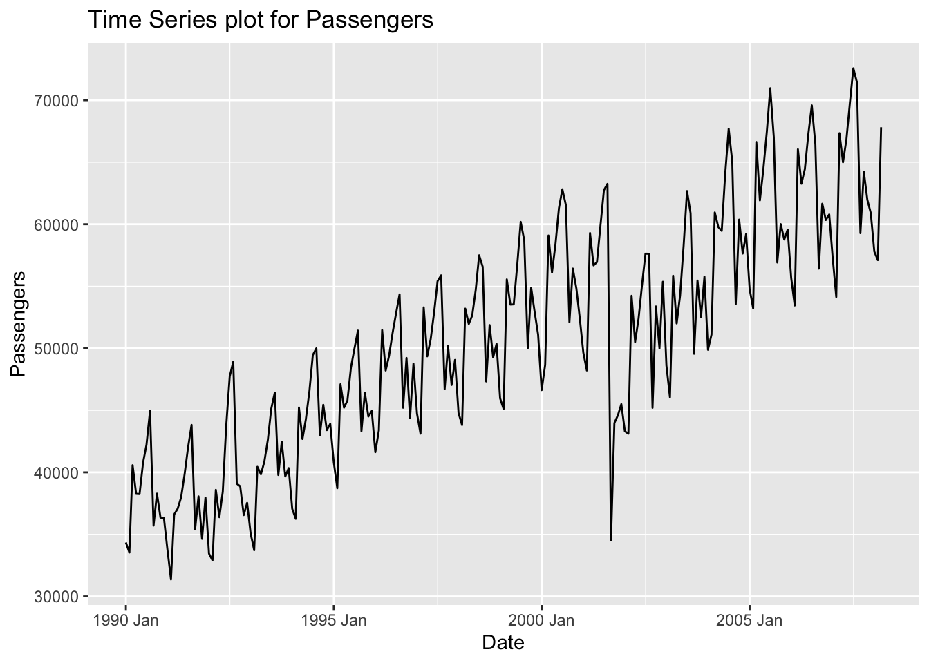
One way to explore time series data is to break the time series down into pieces that summarize different aspects of the possible variation in the dataset. Three common aspects of time series data are trend, seasons, and cycles. Let’s use a dataset to help explain these. Here is a monthly view of the number of airlines passengers in the United States between 1990 and 2008.
Trend
The trend component of a time series is the long term increase or decrease in the dataset. For example, the above airlines dataset has an overall increase in the number of passengers over the years.
Season
The seasonal component of a time series is the repeated pattern over a fixed period of time. For example, the above airlines dataset shows seasonality every 12 observations (12 months) where we see different patterns in summer and holiday times of the year as compared to other times of the year. Seasonality occurs over a fixed and known period of time.
Cycle
Sometimes cycles and season and confused with each other. While seasonal components occur over a fixed period of time, the cycle component of a time series is a rise and fall in the dataset that do not occur with a fixed frequency. The airline dataset above doesn’t really exhibit a cyclical pattern. The drop in number of passengers is due to the September 11 attacks, not to do some business cycle. Those intervention points that sometimes occur in a dataset will be addressed in the dynamic regression section of the website.
A time series decomposition break a series down into the components of trend / cycle (combined together as \(T_t\) ), season (\(S_t\)), and everything left over - the error (\(E_t\)). This decomposition’s seasonal component’s structure is either additive:
\[ Y_t = T_t + S_t + E_t \]
or multiplicative:
\[ Y_t = T_t \times S_t \times E_t \]
For an additive seasonal structure, the magnitude of the variation in the season around the trend/cycle remains relatively constant as seen on the left hand plot below. A multiplicative seasonal component has proportional changes in the variation of the season around the trend / cycle as seen in the right hand plot below.
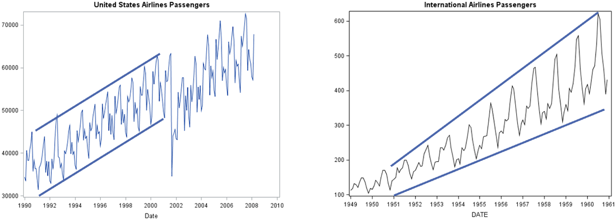
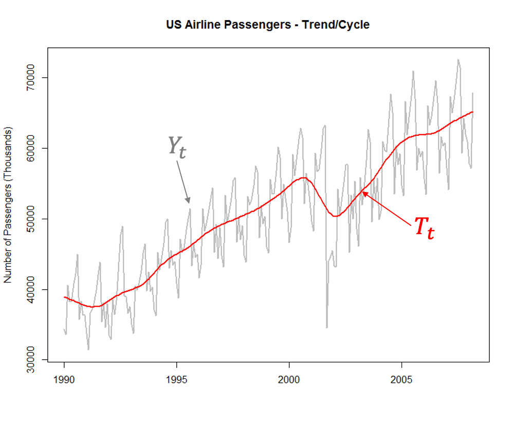
Since our dataset is additive in nature, we will focus our analysis and example on an additive seasonal effect. Once these components are calculated, we can isolate individual pieces to view things a little better. For example, maybe we just want to see the underlying trend / cycle of your data:
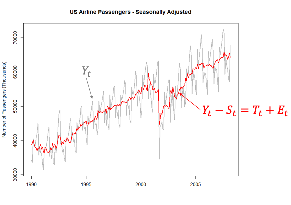
Another popular thing with time series decomposition is to remove the seasonal component, known as a seasonally adjusted time series. This seasonally adjusted series is the original series after subtracting (due to additive season) the seasonal component or taking the previous trend plot and adding in the error component.
Types of Decomposition
There are a variety of different ways to calculate the components of the time series decomposition. Three of the most popular are:
- Classical Decomposition
- X-13 ARIMA-SEATS
- STL (Seasonal and Trend using LOESS) Decomposition
Let’s briefly talk about each.
Classical Decomposition
Classical decomposition is a straight-forward calculation for time series decomposition. It is the default calculation in SAS software. To understand how classical decomposition works, we need to first understand the idea of a rolling / moving average smoothing calculation.
A rolling window average (sometimes called a moving average) smoothing model just averages observations in windows of time.
\[ \hat{Y}_t = \frac{1}{2k + 1} \sum^k_{j = -k} y_{t+j} \]
The \(2k+1\) is called “m” and is referred to as the order of the moving average (an m-MA). Imagine we only had 5 observations in our dataset and we wanted to calculate a 3-MA. We would have the following table:
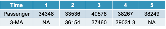
The first value of the 3-MA is not able to be calculated because the data doesn’t have a point before and after it. For the second value of the 3-MA it is just the average of the first 3 values of the data, \((34348 + 33536 + 40578) / 3 = 36154\). The same calculation is done for the remaining observations. As the value of “m” gets larger, the more smooth the model as seen below:
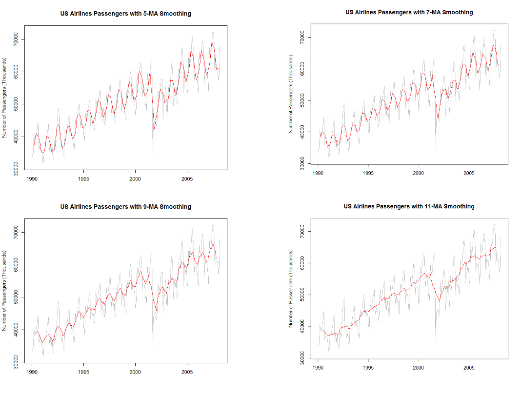
For even values of “m” we typically do moving averages of moving averages to smooth things out even more. The details for this isn’t shown here, but can simply be done by taking a moving average of a previous moving average instead of the original data. For seasonal data with a season length of S, we typically build a 2xS-MA model which uses this double smoothing approach.
For classical decomposition, the trend component in the time series is calculated with these m-MA models. For our dataset, it would use the 2x12-MA smoothing model. Once you have the trend, the seasonal component is calculated by first removing the trend from the original data, \(Y_t - T_t\) in our additive data. From there we literally average these de-trended values for each of the seasonal component pieces to get the seasonal series, \(S_t\). For example, in our dataset, we would average all of the de-trended January values to get our calculation for January. We would continue this for each month. This actually highlights one of the limitations of the classical decomposition approach - that the seasonal component can never change over time. Once you have the trend, \(T_t\), and season, \(S_t\), you subtract those from the original series to get the error, \(E_t = Y_t - T_t - S_t\).
X-13 ARIMA-SEATS
The X-13 ARIMA-SEATS decomposition technique was created by the United States Census Bureau and used by many other countries and in their census statistical analysis. It is the successor to the X-11 and X-12 ARIMA techniques. It uses m-MA smoothing approaches, but also implements time series modeling approaches like ARIMA (discussed in the ARIMA section of the website) and SEATS to help fill in blank values in the m-MA calculation. They do this by forecasting enough values on the end of a series and backcast enough values in the beginning of the series to have enough data points to not have any missing values in the m-MA calculation. They also use m-MA smoothing to calculate the seasonal component as well.
STL Decomposition
Seasonal and trend decomposition using local regression (STL) uses local regression (LOESS) in place of moving averages to calculate both the trend and seasonal components of the series. LOESS is a nonlinear regression technique that uses the simplicity of linear regression applied over small subsets of the data to help it calculate a nonlinear smoothing curve. The smoothing curve is calculated through a weighted least squares regression on a subset of data (window) that moves along the whole series. Let’s look at the flow chart below:
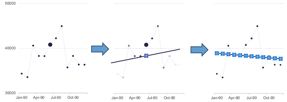
In the first plot above, we isolate out a small window (the first 12 observations). The remaining calculations are done on every window of this size in the data, similar to the m-MA approach described previously. Within this window let’s select a single point as highlighted by the bigger dot. We then uses a weighted linear regression on all the points in the window as shown in the second plot. Any point in the data outside of the window gets no weight in our regression. The closer the observations are to our point of interest the more weight (darker the points above) in the linear regression. We use that linear regression to get a predicted value for that observation which is highlighted by the crossed point above. Imagine we did the exact same process for every point in our dataset as highlighted in the last plot above. We get all of these predicted observations from each of the weight linear regressions (one for every point) and then “connect” them together to form our smoothed curve.
STL decomposition (which is easily implemented in both R and Python) uses LOESS to calculate both the trend, \(T_t\), and seasonal, \(S_t\), components in the decomposition. This allows the seasonal component to adjust over time as compared to the fixed approach of classical decomposition.
Let’s see how to calculate each of these components with our software!
Before exploring our data for modeling, we should explore our dataset and check for any missing values to then correct. This dataset doesn’t have any missing value so this process is skipped here. However, before doing any further exploration we should split our dataset into a train set for modeling and test set for evaluating. In time series we do not randomly split our data into train and test, but split off the final piece for test instead. First, we use the mutate function to create a new date variable made from the Year and Month variables. We use the yearmonth function and the make_date function from the lubridate package. From there we create our tsibble object by using the as_tsibble function where the index for the data is the date variable.
Now that we have our dataset in our modeling format, we can split our data into a train and test split. First we take the tsibble object and use the select function to just keep the Passengers, date, and Month variables. We then use the filter_index function with ~ "2007-03" as an option to use all the data before (and including) March 2007. We will use the same functions to isolate the last year of our data (April 2007 onward).
Code
library(fpp3)

USAirlines <- USAirlines %>%
  mutate(date = yearmonth(lubridate::make_date(Year, Month)))
USAirlines_ts <- as_tsibble(USAirlines, index = date)

train <- USAirlines_ts %>%
  select(Passengers, date, Month) %>%
  filter_index(~ "2007-03")

test <- USAirlines_ts %>%
  select(Passengers, date, Month) %>%
  filter_index("2007-04" ~ .)
Now that we have our training dataset, we can do our time series decomposition. We will use the model function and define a model we will call stl and use the STL function on our Passengers variable. This STL function calculates the STL version of the decomposition as described previously. By default, since we indexed our data by a monthly time index, the function assumes an annual season. This can be changed if we so desire. We then use the components function to print out each of the above components for each observation in our training data. If we want to view these components visually, we can use the autoplot function on the components function output.
Code
dcmp <- train %>%
  model(stl = STL(Passengers))
components(dcmp)
# A dable: 207 x 7 [1M]
# Key: .model [1]
# : Passengers = trend + season_year + remainder
.model date Passengers trend season_year remainder season_adjust
<chr> <mth> <int> <dbl> <dbl> <dbl> <dbl>
1 stl 1990 Jan 34348 39033. -4676. -8.97 39024.
2 stl 1990 Feb 33536 38897. -5842. 481. 39378.
3 stl 1990 Mar 40578 38762. 1238. 578. 39340.
4 stl 1990 Apr 38267 38626. -563. 204. 38830.
5 stl 1990 May 38249 38494. 378. -623. 37871.
6 stl 1990 Jun 40792 38362. 2950. -519. 37842.
7 stl 1990 Jul 42225 38229. 5219. -1223. 37006.
8 stl 1990 Aug 44943 38090. 6551. 302. 38392.
9 stl 1990 Sep 35708 37951. -1956. -287. 37664.
10 stl 1990 Oct 38286 37812. 345. 129. 37941.
# ℹ 197 more rowsCode
components(dcmp) %>% autoplot()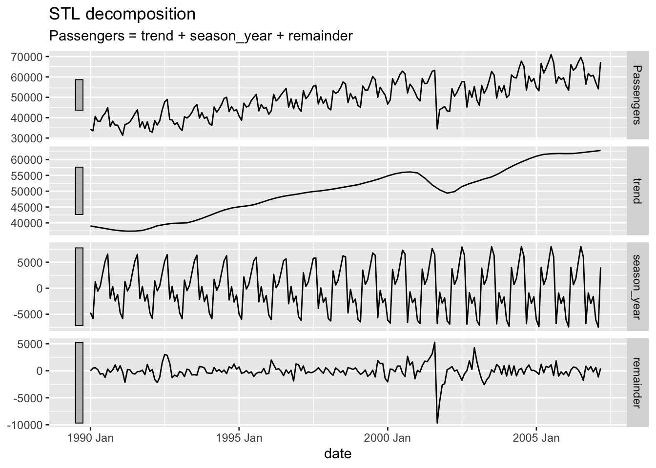
From the decomposition plot above we see the original series, the trend, the seasonal effect, and everything left over. Not surprisingly, the trend is generally going upwards as more passengers use airlines over the years due to population growth. The seasonal piece seems to change slightly over time with more distinct drops between the summer and holiday travel peaks. The error term is not surprising either with the completely unexpected drop due to the September 11 attacks. The grey bars on the sides of the plots show the relative scales of the data compared to each other. The larger a bar is compared to another, the more zoomed in the plot actually is. If two of the grey bars are the same size, then the data is on the same scale in terms of the y-axis.
If you are interested in the other two decomposition techniques, simply replacing STL with either classical_decomposition or SEATS functions in the model function will give you the classical decomposition or X-13 ARIMA-SEATS approaches respectively.
Before exploring our data for modeling, we should explore our dataset and check for any missing values to then correct. This dataset doesn’t have any missing value so this process is skipped here. However, before doing any further exploration we should split our dataset into a train set for modeling and test set for evaluating. In time series we do not randomly split our data into train and test, but split off the final piece for test instead. First, we create our index using the pandas function date_range. We start at January 1990 and go through March 2008 with a frequency of monthly observations. We then take our usair object and make this our index using the pandas function to_datetime.
Code
import pandas as pd
import numpy as np
import matplotlib.pyplot as plt
import statsmodels.api as sm
import seaborn as sns

df = pd.date_range(start = '1/1/1990', end = '3/1/2008', freq = 'MS')
usair.index = pd.to_datetime(df)
Now that we have our dataset with an index, we can split our data into a train and test split. First we take the usair object and use the head function to just keep the first 207 observations which is all the data before (and including) March 2007. We will use the tail function to isolate the last 12 observations of our data (April 2007 onward) to form a year of test data. Next we need to prepare our data for the StatsForecast package in Python. This package requires the train and test data take a very specific format by requiring at least three variables (at the beginning of your dataframe) called ds, unique_id, and y. The unique_id variable specifies different time series you have. Since our dataset is only one time series we are predicting, we will just give this variable a value of 1 for every observation. The ds variable is the date variable. For this we will just use our index from the train dataset. For the y variable we just specify the target variable, here Passengers. We will do the same thing for our test dataset as well.
Code
train = usair.head(207)
test = usair.tail(12)

d = {'unique_id': 1, 'ds': train.index, 'y': train['Passengers']}
train_sf = pd.DataFrame(data = d)

d = {'unique_id': 1, 'ds': test.index, 'y': test['Passengers']}
test_sf = pd.DataFrame(data = d)
Now that we have our training dataset, we can do our time series decomposition. We will use the StatsForecast function and define a model using the MSTL function with a frequency set to monthly data. This MSTL function calculates the STL version of the decomposition as described previously. We then use the fit function with the df = option to specify our training data we want to decompose. We can then use the .fitted_[0,0].model_ functions to print out each of the above components for each observation in our training data. The [0,0] component refers to the first target variable (index of 0 and our only target variable) and the first piece of the output which is the components (again indexed by 0). If we want to view these components visually, we can use the .plot function on the .fitted_[0,0].model_ function output.
Code
from statsforecast import StatsForecast
from statsforecast.models import MSTL

dcmp = StatsForecast(models = [MSTL(season_length = 12)], freq = 'M')
dcmp.fit(df = train_sf)StatsForecast(models=[MSTL])Code
result = dcmp.fitted_[0,0].model_
result
data trend seasonal remainder
0 34348.0 39019.258306 -4656.823649 -14.434657
1 33536.0 38883.031147 -5824.358016 477.326868
2 40578.0 38749.491951 1252.474783 576.033266
3 38267.0 38618.251802 -554.512182 203.260380
4 38249.0 38488.211305 388.631112 -627.842417
.. ... ... ... ...
202 60341.0 62515.681097 -2946.195752 771.514655
203 60791.0 62606.870904 -1594.438482 -221.432422
204 57233.0 62699.163218 -6078.039540 611.876322
205 54140.0 62792.107128 -7499.634204 -1152.472924
206 67342.0 62885.168552 4003.645894 453.185554
[207 rows x 4 columns]Code
dcmp.fitted_[0, 0].model_.plot(subplots=True, grid=True)array([<Axes: >, <Axes: >, <Axes: >, <Axes: >], dtype=object)Code
plt.tight_layout()
plt.show()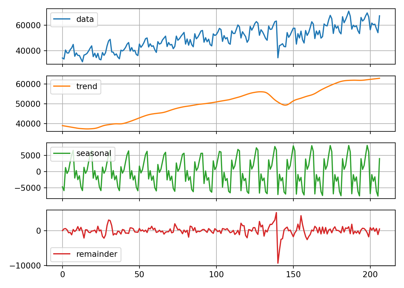
From the decomposition plot above we see the original series, the trend, the seasonal effect, and everything left over. Not surprisingly, the trend is generally going upwards as more passengers use airlines over the years due to population growth. The seasonal piece seems to change slightly over time with more distinct drops between the summer and holiday travel peaks. The error term is not surprising either with the completely unexpected drop due to the September 11 attacks.
Before exploring our data for modeling, we should explore our dataset and check for any missing values to then correct. This dataset doesn’t have any missing value so this process is skipped here. However, before doing any further exploration we should split our dataset into a train set for modeling and test set for evaluating. In time series we do not randomly split our data into train and test, but split off the final piece for test instead. First, we use the mdy function to create a new date variable made from the Year and Month variables. In the mdy function we need to supply a day variable. Since we do not have one, we just place a value of 1 for every date. From there we use the format function to make the date variable into a more readable format.
Code
data work.usair;
    set work.usair;
    date = mdy(Month, 1, Year);
    format date date9.;
run;
Now we can split our data into a train and test split. First we take the dataset and use the where function to just keep the all the data before (and including) March 2007. We will use the same functions to isolate the last year of our data (April 2007 onward).
Code
data work.train;
    set work.usair;
    where date <= '1mar2007'd;
run;

data work.test;
    set work.usair;
    where date > '1mar2007'd;
run;
Now that we have our training dataset, we can do our time series decomposition. By default SAS will provide the classical decomposition. In the PROC TIMESERIES procedure, we use the data =option to provide our training data and the plots = (series decomp) option to ask SAS for a plot of the original data series and a plot of the decomposition. The ID statement is where we provide our date variable and specify our monthly seasonality with the interval = month option. Next, in the VAR statement we provide our target variable, Passengers.
Code
proc timeseries data = work.train plots = (series decomp);
    id date interval = month;
    var Passengers;
run;
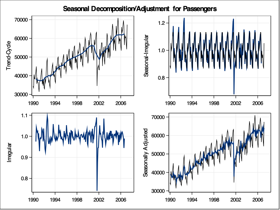
From the decomposition plots above we see the original series, the trend line on the original series, the seasonal effect along with the error term added in, the error term itself (irregular in the plot above), and a seasonally adjusted time series. Not surprisingly, the trend is generally going upwards as more passengers use airlines over the years due to population growth. The seasonal piece remains constant over time due to the classical decomposition technique. The error term is not surprising either with the completely unexpected drop due to the September 11 attacks.