Evaluating Time Series Models
Quick Summary
Prediction Validation
Before we jump too far into modeling, we first need to think about evaluating our models. When it comes to evaluating a model, we need to make sure we evaluate a model in an honest way. Having a model be accurate, essentially predicting the data used to build the model (called training data) is not a good evaluation. Its like taking a test after looking at the answer key. We would expect the model to do well when it has already seen the answer. It is better to have a model that validates well. A well validated model is one that is good at predicting data it has not seen before. This data is called the test data.
Train & Test Split
Before every modeling, we need to split off a piece of data to help us truly evaluate how good our model can do. However, we have to remember that time series data is different than cross-sectional data.
Cross-sectional Data
For cross-sectional data we split off a random subset of our data to help us truly evaluate how good our model is. This is similar to the picture below where any observation can be selected.
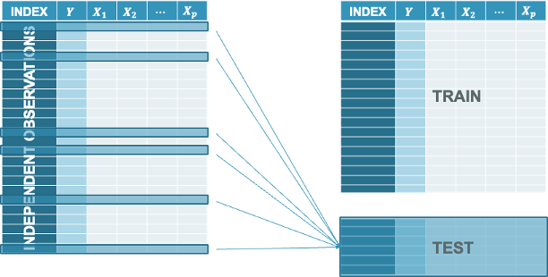
We take this random subset and set it aside as a dataset that we will not touch for modeling. We will only score this dataset with our model to see how good it does. The test dataset is never used to build a model with until the final model is selected. Once you have your final model, you can put all of your data together into one complete dataset and build the same model without any adjustments to what variables or terms are in the model.
Another view of this would be the following scatterplot where on the left hand side we have the full data with the test data set point highlighted in a lighter color. On the right was have just the training dataset that will be used for model building.
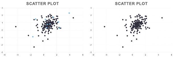
We are essentially removing these data points for our model building so we can only focus on the training dataset. Once our model is done, we will see how good our model does at predicting those data points to see how well we actually did.
What if that random subset of your data that you selected for training just be random chance was easy to predict? What if it was hard to predict by random chance. Due to this possibility, another option for splitting with cross-sectional data is called cross-validation. In cross-validation you still have a random subset of data you put aside. For this example, let’s say it is 10% of your data. However, you don’t stop at one subset. You go through the whole process and build a model on 90% of your data (training) and evaluate on the 10% you left aside. Then you repeat this process again with a different random 10% subset. The only condition is that this new 10% cannot contain any of the observations that were in the original 10% you set aside.
You repeat this process until you cover the whole dataset where every observation belonged to one of the 10% subsets that you put aside. Essentially, you do the process 10 times because you set out 10%.
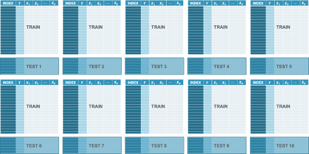
Once this is done, you average together the metrics on these separate test datasets to get a better idea of how you did.
Time Series Data
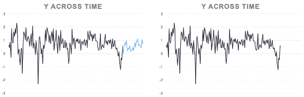
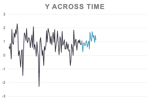
In time series data we cannot do a random subset. If each observation depends on the previous one for time series, then you can’t just remove random observations. In time series is it not random in how we select our subset for the test dataset. It is typically the last piece of the data. We build our model on an earlier piece of the data and try to forecast the last piece that our model has not seen.
We take this specific subset and set it aside as a dataset that we will not touch for modeling. We will only score this dataset with our model to see how good it does. The test dataset is never used to build a model with until the final model is selected. Once you have your final model, you can put all of your data together into one complete dataset and build the same model without any adjustments to what variables or terms are in the model.
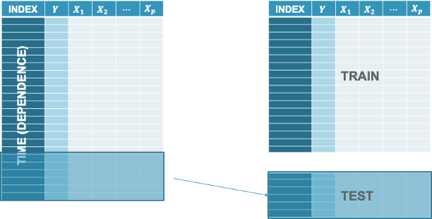
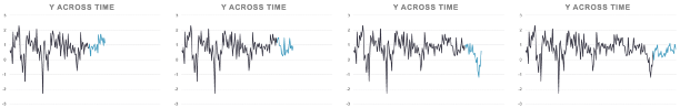
Another view of this would be the following plot where on the left hand side we have the full data with the test data set point highlighted in a lighter color at the end of the time series. On the right was have just the training dataset that will be used for model building.
We are essentially removing these data points for our model building so we can only focus on the training dataset. Once our model is done, we will see how good our model does at forecasting those data points to see how well we actually did.
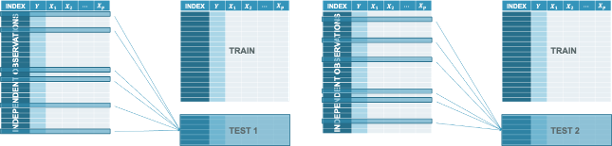
Similar to cross-sectional data, time series has something similar to the cross-validation variation on the typical train and test splitting process. In time series we call it rolling hold-out samples or rolling test samples. Here we take a much earlier piece of the data and still set aside a small portion for testing. We build a model on this smaller training and evaluate on the small testing to calculate a metric to see how well we do.
Next, we take the piece you just used for testing and add it back into the training data and build a model on that while keeping the next little slice of data out for testing. Again, we evaluate our new model on this new test dataset and record our model metric. The idea of the rolling window is that we keep this process going by gradually adding in small pieces of the dataset for model building and evaluating on the next small piece until we get to the end of the dataset.
Then we just average all of our test dataset metrics to see how well we did. It is similar to cross-validation, but with a time series spin on it.
Evaluation Metrics
Now that we have our test dataset (or many test datasets with rolling hold-out samples), we need metrics to evaluate our models with. There are seemingly an endless quantity of metrics people have proposed over the years. Four of the most popular metrics are the following:
- Mean Absolute Error (MAE)
- Mean Squared Error (MSE)
- Mean Absolute Percentage Error (MAPE)
- Symmetric Mean Absolute Percentage Error (sMAPE)
These metrics fall into two broader categories - scale dependent and symmetric vs. Scale independent and asymmetric.
Scale Dependent and Symmetric
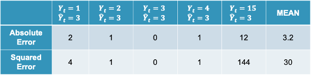
The first two metrics are the MAE and MSE:
Mean Absolute Error (MAE):
\[ MAE = \frac{1}{n} \sum_{t=1}^n |Y_t - \hat{Y}_t| \]
Mean Squared Error (MSE):
\[ MSE = \frac{1}{n} \sum_{t=1}^n (Y_t - \hat{Y}_t)^2 \]
These first two metrics above are both scale dependent and symmetric. Scale dependent metrics are metrics that can only be compared to data with similar values for the data points. For example, we cannot compare a model trying to predict the price of a car with another model trying to predict the GDP of a country with MAE. An average error of $100,000 might be good for a model predicting GDP, but not as good for a model predicting price of a car. A symmetric metric is a metric that has the same meaning if the prediction is above the actual value as below the actual value. Again, for example, an error of $10,000 above a prediction is the same as an error $10,000 below a prediction.
Scale Independent and Asymmetric
The final two metrics are the MAPE and sMAPE:
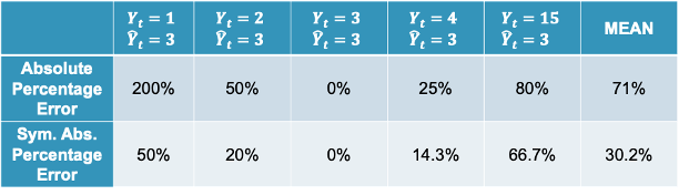
Mean Absolute Percentage Error (MAPE):
\[ MAPE = \frac{1}{n} \sum_{t=1}^n |\frac{Y_t - \hat{Y}_t}{Y_t}| \]
Symmetric MAPE (sMAPE):
\[ sMAPE = \frac{1}{n} \sum_{t=1}^n \frac{|Y_t - \hat{Y}_t|}{|Y_t| + |\hat{Y}_t|} \]
These final two metrics above are both scale independent and asymmetric. Scale independent metrics are metrics that can be compared to data with any values for the data points. For example, we can compare a model trying to predict the price of a car with another model trying to predict the GDP of a country with MAPE. An average percentage error of 4% would be a worse model in context compared to a model with an average percentage error of 2.5%. An asymmetric metric is a metric that has a different meaning if the prediction is above the actual value as below the actual value. For example, a 5% error above is not the same as a 5% error below. It may be weird to think that a metric called Symmetric MAPE is asymmetric, but it is just more symmetric than the traditional MAPE, not completely symmetric.