It is easy to generalize the binary logistic regression model to the ordinal logistic regression model. However, we need to change the underlying model and math slightly to extend to nominal target variables.
In binary logistic regression we are calculating the probability that an observation has an event. In ordinal logistic regression we are calculating the probability that an observation has at most that event in an ordered list of outcomes. In nominal (or multinomial) logistic regression we are calculating the probability that an observation has a specific event in an unordered list of events.
We will be using the alligator data set to model the association between various factors and alligator food choices - fish, invertebrate, birds, reptiles, and other. The variables in the data set are the following:
Variable
Description
size
small (< 2.3 meters) or large (> 2.3 meters)
lake
lake captured (George, Hancock, Oklawaha, Trafford)
gender
male or female
count
number of observations with characteristics
Generalized Logit Model
Instead of modeling the typical logit from binary or ordinal logistic regression, we will model the generalized logits. These generalized logits are built off target variables with \(m\) categories. The first logit will summarize the probability of the first category compared to the probability of the reference category. The second logit will summarize the probability of the second category compared to the probability of the reference. This continues \(m-1\) times as the last logit compares the \(m-1\) category to the reference category. In essence, with a target variable with \(m\) categories, we are building \(m-1\) logistic regressions. However, unlike the ordinal logistic regression where we have different intercepts with the same slope parameters, in nominal logistic regression we have both different intercepts and different slope parameters for each model.
The logits are also not traditional logits. Instead of the natural log of the odds, they are natural logs of relative risks - ratios of two probabilities that do not sum to 1.
Let’s see how to build these generalized logit models in each of our softwares!
The data set is structured slightly differently than previous data sets. Let’s examine the first 10 observations with the head function and the n = 10 option.
Code
head(gator, n =10)
            size         food    lake gender count
1  <= 2.3 meters         Fish Hancock   Male     7
2  <= 2.3 meters Invertebrate Hancock   Male     1
3  <= 2.3 meters        Other Hancock   Male     5
4   > 2.3 meters         Fish Hancock   Male     4
5   > 2.3 meters         Bird Hancock   Male     1
6   > 2.3 meters        Other Hancock   Male     2
7  <= 2.3 meters         Fish Hancock Female    16
8  <= 2.3 meters Invertebrate Hancock Female     3
9  <= 2.3 meters      Reptile Hancock Female     2
10 <= 2.3 meters         Bird Hancock Female     2
Notice the count variable. In the first observation we can see that we have seven alligators that are small, males captured on Lake Hancock and eat fish. The same applies for each row in our data set. Even with only 56 rows in our data set, we have 219 observations based on the counts.
To account for the multiple counts in a single row of our data set we use the weight = option in the vglm function (like we saw with ordinal logistic regression) with the count variable. The formula structure for the vglm function is the same as with previous functions in logistic regression. The target variable food needs to be turned into a factor with the factor function. Instead of cumulative for the family = option like we had in ordinal logistic regression, we use the family = multinomial option. We set the reference level specified with the refLevel option so we know what R chooses. By default the vglm function will use the last level of the variable. Here, our reference level is fish because it has the largest proportion of our observations. Similar to before, the summary function will display our needed results.
Code
gator$food <-factor(gator$food)library(VGAM)glogit.model <-vglm(food ~ size + lake + gender,data = gator, family =multinomial(refLevel ="Fish"),weight = count)summary(glogit.model)
Call:
vglm(formula = food ~ size + lake + gender, family = multinomial(refLevel = "Fish"),
    data = gator, weights = count)

Coefficients:
                   Estimate Std. Error z value Pr(>|z|)
(Intercept):1      -2.43211    0.77066      NA       NA
(Intercept):2       0.16902    0.37875   0.446  0.65541
(Intercept):3      -1.43073    0.53809  -2.659  0.00784 **
(Intercept):4      -3.41604    1.08513      NA       NA
size> 2.3 meters:1  0.73024    0.65228   1.120  0.26292
size> 2.3 meters:2 -1.33626    0.41119  -3.250  0.00116 **
size> 2.3 meters:3 -0.29058    0.45993  -0.632  0.52752
size> 2.3 meters:4  0.55704    0.64661   0.861  0.38898
lakeHancock:1       0.57527    0.79522   0.723  0.46943
lakeHancock:2      -1.78051    0.62321  -2.857  0.00428 **
lakeHancock:3       0.76658    0.56855   1.348  0.17756
lakeHancock:4       1.12946    1.19280   0.947  0.34369
lakeOklawaha:1     -0.55035    1.20987  -0.455  0.64919
lakeOklawaha:2      0.91318    0.47612   1.918  0.05511 .
lakeOklawaha:3      0.02606    0.77777   0.034  0.97327
lakeOklawaha:4      2.53026    1.12212   2.255  0.02414 *
lakeTrafford:1      1.23699    0.86610   1.428  0.15323
lakeTrafford:2      1.15582    0.49279   2.345  0.01900 *
lakeTrafford:3      1.55776    0.62567   2.490  0.01278 *
lakeTrafford:4      3.06105    1.12973   2.710  0.00674 **
genderMale:1       -0.60643    0.68885  -0.880  0.37867
genderMale:2       -0.46296    0.39552  -1.171  0.24180
genderMale:3       -0.25257    0.46635  -0.542  0.58810
genderMale:4       -0.62756    0.68528  -0.916  0.35978
---
Signif. codes:  0 '***' 0.001 '**' 0.01 '*' 0.05 '.' 0.1 ' ' 1

Names of linear predictors: log(mu[,1]/mu[,2]), log(mu[,3]/mu[,2]),
log(mu[,4]/mu[,2]), log(mu[,5]/mu[,2])

Residual deviance: 537.8655 on 200 degrees of freedom

Log-likelihood: -268.9327 on 200 degrees of freedom

Number of Fisher scoring iterations: 6

Warning: Hauck-Donner effect detected in the following estimate(s):
'(Intercept):1', '(Intercept):4'


Reference group is level  2  of the response
In the output above we see similar things to the output we have seen previously. R summarizes the parameter estimates, their standard errors, and corresponding p-values. The main difference in the parameter estimates is the multiple intercepts and slope coefficients for each variable. Since we have five levels of our target variable we have four logistic regression models and therefore four intercepts and four slope parameters for each variable.
The data set is structured slightly differently than previous data sets. Let’s examine the first 10 observations with the head function and the n = 10 option.
Code
gator.head(n =10)
            size          food     lake  gender  count
0  <= 2.3 meters          Fish  Hancock    Male      7
1  <= 2.3 meters  Invertebrate  Hancock    Male      1
2  <= 2.3 meters         Other  Hancock    Male      5
3   > 2.3 meters          Fish  Hancock    Male      4
4   > 2.3 meters          Bird  Hancock    Male      1
5   > 2.3 meters         Other  Hancock    Male      2
6  <= 2.3 meters          Fish  Hancock  Female     16
7  <= 2.3 meters  Invertebrate  Hancock  Female      3
8  <= 2.3 meters       Reptile  Hancock  Female      2
9  <= 2.3 meters          Bird  Hancock  Female      2
Notice the count variable. In the first observation we can see that we have seven alligators that are small, males captured on Lake Hancock and eat fish. The same applies for each row in our data set. Even with only 56 rows in our data set, we have 219 observations based on the counts.
We need to expand our dataset to run the analysis in Python. To do this we just use the repeat and index attributes of the gator dataset. Let’s see the new dataset!
            size          food     lake gender  count
0  <= 2.3 meters          Fish  Hancock   Male      7
1  <= 2.3 meters          Fish  Hancock   Male      7
2  <= 2.3 meters          Fish  Hancock   Male      7
3  <= 2.3 meters          Fish  Hancock   Male      7
4  <= 2.3 meters          Fish  Hancock   Male      7
5  <= 2.3 meters          Fish  Hancock   Male      7
6  <= 2.3 meters          Fish  Hancock   Male      7
7  <= 2.3 meters  Invertebrate  Hancock   Male      1
8  <= 2.3 meters         Other  Hancock   Male      5
9  <= 2.3 meters         Other  Hancock   Male      5
Now the dataset is in workable format lengthwise. However, the MNLogit function we need to use for nominal logistic regression doesn’t have a from_formula attribute. Therefore, we need to get all of our predictor variables into a workable format for modeling. Since we have categorical variables, we need to dummy code them. The from_formula framework in earlier sections did that for us before. To do that ourselves we use the get_dummies function on the three categorical variables - size, lake, and gender. We drop the target variable food from this function as well as the original count variable. This set of dummy encoded variables now serves as our X matrix. The target variable food is our y. These are the inputs into the MNLogit function. We use the typical summary function to view the results.
Optimization terminated successfully.
         Current function value: 1.320942
         Iterations 7
Code
glogit_model.summary()
MNLogit Regression Results
Dep. Variable:
food
No. Observations:
219
Model:
MNLogit
Df Residuals:
199
Method:
MLE
Df Model:
16
Date:
Mon, 24 Jun 2024
Pseudo R-squ.:
0.04267
Time:
19:34:02
Log-Likelihood:
-289.29
converged:
True
LL-Null:
-302.18
Covariance Type:
nonrobust
LLR p-value:
0.05705
food=Fish
coef
std err
z
P>|z|
[0.025
0.975]
size_> 2.3 meters
0.1289
0.520
0.248
0.804
-0.890
1.147
lake_Hancock
1.2721
0.515
2.470
0.014
0.262
2.282
lake_Oklawaha
1.6785
1.087
1.544
0.123
-0.452
3.809
lake_Trafford
-0.2345
0.699
-0.335
0.737
-1.605
1.136
gender_Male
1.6597
0.529
3.137
0.002
0.623
2.697
food=Invertebrate
coef
std err
z
P>|z|
[0.025
0.975]
size_> 2.3 meters
-1.4893
0.607
-2.452
0.014
-2.680
-0.299
lake_Hancock
-0.2610
0.695
-0.375
0.707
-1.623
1.101
lake_Oklawaha
2.9920
1.077
2.778
0.005
0.881
5.103
lake_Trafford
1.3399
0.674
1.989
0.047
0.020
2.660
gender_Male
1.2814
0.564
2.274
0.023
0.177
2.386
food=Other
coef
std err
z
P>|z|
[0.025
0.975]
size_> 2.3 meters
-0.4827
0.585
-0.825
0.409
-1.629
0.664
lake_Hancock
0.9376
0.550
1.705
0.088
-0.140
2.015
lake_Oklawaha
0.9792
1.205
0.813
0.416
-1.383
3.341
lake_Trafford
0.6902
0.718
0.962
0.336
-0.716
2.097
gender_Male
0.7256
0.584
1.243
0.214
-0.419
1.870
food=Reptile
coef
std err
z
P>|z|
[0.025
0.975]
size_> 2.3 meters
-0.0520
0.604
-0.086
0.931
-1.236
1.132
lake_Hancock
-0.5174
0.748
-0.692
0.489
-1.983
0.949
lake_Oklawaha
1.9040
1.123
1.696
0.090
-0.297
4.105
lake_Trafford
0.6295
0.739
0.852
0.394
-0.818
2.077
gender_Male
0.1429
0.639
0.223
0.823
-1.110
1.396
In the output above we see similar things to the output we have seen previously. Python summarizes the parameter estimates and their standard errors. The main difference in the parameter estimates is the multiple intercepts and slope coefficients for each variable. Since we have five levels of our target variable we have four logistic regression models and therefore four intercepts and four slope parameters for each variable.
The data set is structured slightly differently than previous data sets. Let’s examine the first 10 observations with PROC PRINT and the obs = 10 option.
Code
proc print data=logistic.gator (obs =10);run;
Notice the count variable. In the first observation we can see that we have seven alligators that are small, males captured on Lake Hancock and eat fish. The same applies for each row in our data set. Even with only 56 rows in our data set, we have 219 observations based on the counts.
To account for the multiple counts in a single row of our data set we use the FREQ statement in PROC LOGISTIC with the count variable. The CLASS statement still defines our categorical variables for lake, size, and gender. The target variable food has a reference level specified with the ref = option. Here, our reference level is fish because it has the largest proportion of our observations. The link = glogit option tells PROC LOGISTIC to use the generalized logit model.
Code
proc logistic data=Logistic.Gator plot(only)=oddsratio(range=clip); freq count; class lake(param=ref ref='George') size(param=ref ref='<= 2.3 meters') gender(param=ref ref='Male'); model food(ref='Fish') = lake size gender / link=glogit clodds=pl; title 'Model on Alligator Food Choice';run;quit;
In the output above we see similar things to the output we have seen previously. PROC LOGISTIC summarizes the model used, the number of observations read and used in the model, and builds a frequency table for our target variable. It then summarizes the categorical variables created in the CLASS statement followed by telling us that the model converged. It also provides us with the same global tests, type 3 analysis of effects, parameter estimates, and odds ratios we have discussed in previous sections. The main difference in the parameter estimates is the multiple intercepts and slope coefficients for each variable. Since we have five levels of our target variable we have four logistic regression models and therefore four intercepts and four slope parameters for each variable.
Interpretation
Similar to binary and ordinal logistic regression models, we exponentiate the coefficients in our nominal logistic regression model to make them interpretable. However, the interpretation changes since these are not odds ratios anymore, but relative risk ratios. Let’s use the coefficient for the birds model and the size variable. It would be incorrect to say that the probability of eating birds is 2.076 times as likely for large alligators compared to small alligators. The correct interpretation would be that the predicted relative probability of eating birds rather than fish is 2.076 times as likely in large alligators compared to small alligators. Notice how our interpretation is in comparison to the reference level. Sometimes these are called conditional interpretations.
Let’s see how to get these from each of our softwares!
As with previous models, we just need to use the exp function to exponentiate the coefficients from our nominal logistic regression model to get the relative risk ratios.
As with previous models, we just need to use the exp function from numpy to exponentiate the coefficients from our nominal logistic regression model to get the relative risk ratios.
Code
import numpy as np100*(np.exp(glogit_model.params)-1)
By default, SAS produces the odds ratio table that shows the exponentiated coefficients. Even those these are not actually considered odds ratios in the traditional sense, the calculation in the odds ratio table is still correct.
Code
ods html select CLOddsPL;proc logistic data=Logistic.Gator plot(only)=oddsratio(range=clip); freq count; class lake(param=ref ref='George') size(param=ref ref='<= 2.3 meters') gender(param=ref ref='Male'); model food(ref='Fish') = lake size gender / link=glogit clodds=pl; title 'Model on Alligator Food Choice';run;quit;
Predictions & Diagnostics
Nominal logistic regression has a lot of similarities to binary logistic regression:
Multicollinearity still exists
Non-convergence problems still exists
AIC and BIC metrics can still be calculated
Generalized \(R^2\) remains the same
There are some inherent differences though between binary and nominal logistic regression. A lot of the diagnostics cannot be calculated for multinomial logistic regression. ROC curves and residuals cannot typically be calculated because there is actually more than one logistic regression occurring.
Predicted probabilities are actually for each category though. Let’s see how we can get predicted probabilities from each of our softwares!
In R we have the same process of getting predicted probabilities in multinomial logistic regression as we did for binary and ordinal logistic regression. The predict function will score any data set. The type = response option is used to get individual predicted probabilities for each category.
Code
pred_probs <-predict(glogit.model, newdata = gator, type ="response")head(pred_probs)
The five variables are the individual predicted probabilities for each of the categories of our target variable. Unlike binary logistic regression where we typically did not use a cut-off of 0.5 to determine which category we predict, in nominal logistic regression we typically pick the category with the highest probability as our predicted category.
Accuracy is typically not as high in logistic regressions with more than two categories because there are more chances for incorrect predictions.
In R we have the same process of getting predicted probabilities in multinomial logistic regression as we did for binary and ordinal logistic regression. The predict function will score any data set.
The five variables are the individual predicted probabilities for each of the categories of our target variable. Unlike binary logistic regression where we typically did not use a cut-off of 0.5 to determine which category we predict, in multinomial logistic regression we typically pick the category with the highest probability as our predicted category.
Accuracy is typically not as high in logistic regressions with more than two categories because there are more chances for incorrect predictions.
In PROC LOGISTIC we have the same process of getting predicted probabilities in multinomial logistic regression as we did for binary and ordinal logistic regression. The OUTPUT statement will score the training set, while the SCORE statement will score the validation data set. The predprobs = I option is used to get individual predicted probabilities for each category.
Code
ods html select none;proc logistic data=Logistic.Gator plot(only)=oddsratio(range=clip); freq count; class lake(param=ref ref='George') size(param=ref ref='<= 2.3 meters') gender(param=ref ref='Male'); model food(ref='Fish') = lake size gender / link=glogit clodds=pl; output out=pred predprobs=I; title 'Model on Alligator Food Choice';run;quit;ods html select all;proc print data=pred (obs =5);run;proc freq data=pred; weight count; tables _FROM_*_INTO_; title 'Crosstabulation of Observed by Predicted Responses';run;
The IP variables are the individual predicted probabilities for each of the categories of our target variable. Unlike binary logistic regression where we typically did not use a cut-off of 0.5 to determine which category we predict, in multinomial logistic regression we typically pick the category with the highest probability as our predicted category. The FROM and INTO variables are the actual target variable category and the predicted category for the target respectively.
To see how the predicted categories compare with the actual target categories we can use PROC FREQ with a TABLES statement on the FROM and INTO variables.
Accuracy is typically not as high in logistic regressions with more than two categories because there are more chances for incorrect predictions.
Source Code
---title: "Multinomial Logistic Regression"format: html: code-fold: show code-tools: trueeditor: visual---```{r}#| include: false#| warning: falsegator <-read.csv(file ="~/My Drive (adlabarr@ncsu.edu)/IAA/Courses/IAA/Logistic Regression/Code Files/Logistic-new/data/gator.csv", header =TRUE)``````{python}#| include: falsegator = r.gator```# Nominal Target VariableIt is easy to generalize the binary logistic regression model to the ordinal logistic regression model. However, we need to change the underlying model and math slightly to extend to nominal target variables.In binary logistic regression we are calculating the probability that an observation has an event. In ordinal logistic regression we are calculating the probability that an observation has at most that event in an ordered list of outcomes. In nominal (or multinomial) logistic regression we are calculating the probability that an observation has a specific event in an unordered list of events.We will be using the alligator data set to model the association between various factors and alligator food choices - fish, invertebrate, birds, reptiles, and other. The variables in the data set are the following:| Variable | Description ||----------|-----------------------------------------------------|| size | small (\< 2.3 meters) or large (\> 2.3 meters) || lake | lake captured (George, Hancock, Oklawaha, Trafford) || gender | male or female || count | number of observations with characteristics |# Generalized Logit ModelInstead of modeling the typical logit from binary or ordinal logistic regression, we will model the generalized logits. These generalized logits are built off target variables with $m$ categories. The first logit will summarize the probability of the first category compared to the probability of the reference category. The second logit will summarize the probability of the second category compared to the probability of the reference. This continues $m-1$ times as the last logit compares the $m-1$ category to the reference category. In essence, with a target variable with $m$ categories, we are building $m-1$ logistic regressions. However, unlike the ordinal logistic regression where we have different intercepts with the same slope parameters, in nominal logistic regression we have both different intercepts and different slope parameters for each model.The logits are also not traditional logits. Instead of the natural log of the odds, they are natural logs of relative risks - ratios of two probabilities that do not sum to 1.Let's see how to build these generalized logit models in each of our softwares!::: {.panel-tabset .nav-pills}## RThe data set is structured slightly differently than previous data sets. Let's examine the first 10 observations with the `head` function and the `n = 10` option.```{r}head(gator, n =10)```Notice the *count* variable. In the first observation we can see that we have seven alligators that are small, males captured on Lake Hancock and eat fish. The same applies for each row in our data set. Even with only 56 rows in our data set, we have 219 observations based on the counts.To account for the multiple counts in a single row of our data set we use the `weight =` option in the `vglm` function (like we saw with ordinal logistic regression) with the *count* variable. The formula structure for the `vglm` function is the same as with previous functions in logistic regression. The target variable *food* needs to be turned into a factor with the `factor` function. Instead of `cumulative` for the `family =` option like we had in ordinal logistic regression, we use the `family = multinomial` option. We set the reference level specified with the `refLevel` option so we know what R chooses. By default the `vglm` function will use the last level of the variable. Here, our reference level is fish because it has the largest proportion of our observations. Similar to before, the `summary` function will display our needed results.```{r}#| message: falsegator$food <-factor(gator$food)library(VGAM)glogit.model <-vglm(food ~ size + lake + gender,data = gator, family =multinomial(refLevel ="Fish"),weight = count)summary(glogit.model)```In the output above we see similar things to the output we have seen previously. R summarizes the parameter estimates, their standard errors, and corresponding p-values. The main difference in the parameter estimates is the multiple intercepts and slope coefficients for each variable. Since we have five levels of our target variable we have four logistic regression models and therefore four intercepts and four slope parameters for each variable.## PythonThe data set is structured slightly differently than previous data sets. Let's examine the first 10 observations with the `head` function and the `n = 10` option.```{python}gator.head(n =10)```Notice the *count* variable. In the first observation we can see that we have seven alligators that are small, males captured on Lake Hancock and eat fish. The same applies for each row in our data set. Even with only 56 rows in our data set, we have 219 observations based on the counts.We need to expand our dataset to run the analysis in Python. To do this we just use the `repeat` and `index` attributes of the `gator` dataset. Let's see the new dataset!```{python}gator = gator.loc[gator.index.repeat(gator['count'])]gator = gator.reset_index(drop =True)gator.head(n =10)```Now the dataset is in workable format lengthwise. However, the `MNLogit` function we need to use for nominal logistic regression doesn't have a `from_formula` attribute. Therefore, we need to get all of our predictor variables into a workable format for modeling. Since we have categorical variables, we need to dummy code them. The `from_formula` framework in earlier sections did that for us before. To do that ourselves we use the `get_dummies` function on the three categorical variables - *size*, *lake*, and *gender*. We drop the target variable *food* from this function as well as the original *count* variable. This set of dummy encoded variables now serves as our X matrix. The target variable *food* is our y. These are the inputs into the `MNLogit` function. We use the typical `summary` function to view the results.```{python}import pandas as pdimport statsmodels.api as smay = gator['food']X = pd.get_dummies(data = gator, columns = ['size', 'lake', 'gender'], drop_first =True).drop(columns = ['food', 'count'])glogit_model = sma.MNLogit(y, X).fit()glogit_model.summary()```In the output above we see similar things to the output we have seen previously. Python summarizes the parameter estimates and their standard errors. The main difference in the parameter estimates is the multiple intercepts and slope coefficients for each variable. Since we have five levels of our target variable we have four logistic regression models and therefore four intercepts and four slope parameters for each variable.## SASThe data set is structured slightly differently than previous data sets. Let's examine the first 10 observations with PROC PRINT and the `obs = 10` option.```{r}#| eval: falseproc print data=logistic.gator (obs =10);run;```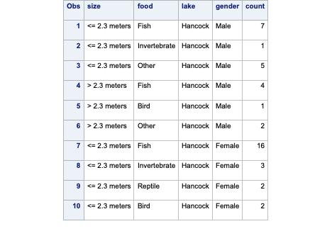{fig-align="center" width="6in"}Notice the *count* variable. In the first observation we can see that we have seven alligators that are small, males captured on Lake Hancock and eat fish. The same applies for each row in our data set. Even with only 56 rows in our data set, we have 219 observations based on the counts.To account for the multiple counts in a single row of our data set we use the FREQ statement in PROC LOGISTIC with the *count* variable. The CLASS statement still defines our categorical variables for *lake*, *size*, and *gender*. The target variable *food* has a reference level specified with the `ref =` option. Here, our reference level is fish because it has the largest proportion of our observations. The `link = glogit` option tells PROC LOGISTIC to use the generalized logit model.```{r}#| eval: falseproc logistic data=Logistic.Gator plot(only)=oddsratio(range=clip); freq count; class lake(param=ref ref='George') size(param=ref ref='<= 2.3 meters') gender(param=ref ref='Male'); model food(ref='Fish') = lake size gender / link=glogit clodds=pl; title 'Model on Alligator Food Choice';run;quit;```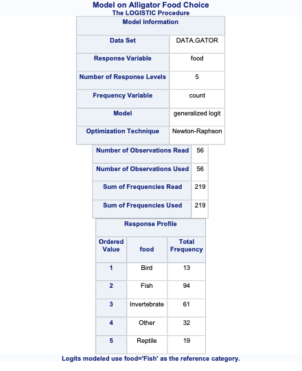{fig-align="center" width="6in"}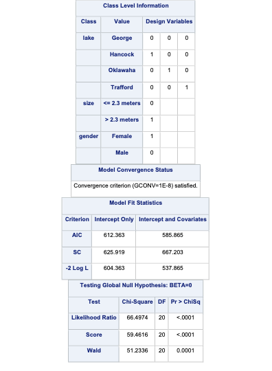{fig-align="center" width="6in"}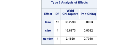{fig-align="center" width="6in"}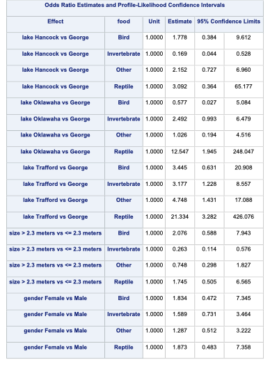{fig-align="center" width="6in"}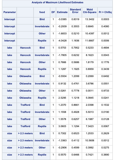{fig-align="center" width="6in"}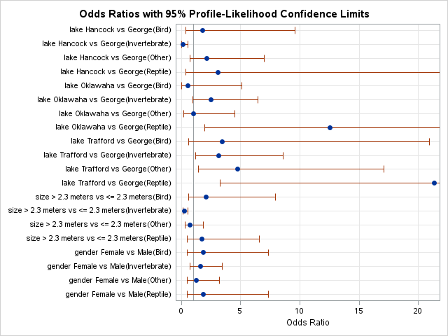{fig-align="center"}In the output above we see similar things to the output we have seen previously. PROC LOGISTIC summarizes the model used, the number of observations read and used in the model, and builds a frequency table for our target variable. It then summarizes the categorical variables created in the CLASS statement followed by telling us that the model converged. It also provides us with the same global tests, type 3 analysis of effects, parameter estimates, and odds ratios we have discussed in previous sections. The main difference in the parameter estimates is the multiple intercepts and slope coefficients for each variable. Since we have five levels of our target variable we have four logistic regression models and therefore four intercepts and four slope parameters for each variable.:::# InterpretationSimilar to binary and ordinal logistic regression models, we exponentiate the coefficients in our nominal logistic regression model to make them interpretable. However, the interpretation changes since these are not odds ratios anymore, but relative risk ratios. Let's use the coefficient for the birds model and the *size* variable. It would be **incorrect** to say that the probability of eating birds is 2.076 times as likely for large alligators compared to small alligators. The **correct** interpretation would be that the predicted **relative probability** of eating birds **rather than fish** is 2.076 times as likely in large alligators compared to small alligators. Notice how our interpretation is in comparison to the reference level. Sometimes these are called **conditional** interpretations.Let's see how to get these from each of our softwares!::: {.panel-tabset .nav-pills}## RAs with previous models, we just need to use the `exp` function to exponentiate the coefficients from our nominal logistic regression model to get the relative risk ratios.```{r}100*(exp(coef(glogit.model))-1)```## PythonAs with previous models, we just need to use the `exp` function from `numpy` to exponentiate the coefficients from our nominal logistic regression model to get the relative risk ratios.```{python}import numpy as np100*(np.exp(glogit_model.params)-1)```## SASBy default, SAS produces the odds ratio table that shows the exponentiated coefficients. Even those these are not actually considered odds ratios in the traditional sense, the calculation in the odds ratio table is still correct.```{r}#| eval: falseods html select CLOddsPL;proc logistic data=Logistic.Gator plot(only)=oddsratio(range=clip); freq count; class lake(param=ref ref='George') size(param=ref ref='<= 2.3 meters') gender(param=ref ref='Male'); model food(ref='Fish') = lake size gender / link=glogit clodds=pl; title 'Model on Alligator Food Choice';run;quit;```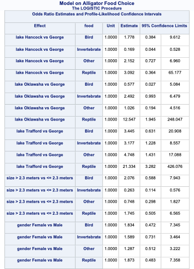{fig-align="center" width="6in"}:::# Predictions & DiagnosticsNominal logistic regression has a lot of similarities to binary logistic regression:- Multicollinearity still exists- Non-convergence problems still exists- AIC and BIC metrics can still be calculated- Generalized $R^2$ remains the sameThere are some inherent differences though between binary and nominal logistic regression. A lot of the diagnostics cannot be calculated for multinomial logistic regression. ROC curves and residuals cannot typically be calculated because there is actually more than one logistic regression occurring.Predicted probabilities are actually for each category though. Let's see how we can get predicted probabilities from each of our softwares!::: {.panel-tabset .nav-pills}## RIn R we have the same process of getting predicted probabilities in multinomial logistic regression as we did for binary and ordinal logistic regression. The `predict` function will score any data set. The `type = response` option is used to get individual predicted probabilities for each category.```{r}pred_probs <-predict(glogit.model, newdata = gator, type ="response")head(pred_probs)```The five variables are the individual predicted probabilities for each of the categories of our target variable. Unlike binary logistic regression where we typically did not use a cut-off of 0.5 to determine which category we predict, in nominal logistic regression we typically pick the category with the highest probability as our predicted category.Accuracy is typically not as high in logistic regressions with more than two categories because there are more chances for incorrect predictions.## PythonIn R we have the same process of getting predicted probabilities in multinomial logistic regression as we did for binary and ordinal logistic regression. The `predict` function will score any data set.```{python}glogit_model.predict(X)```The five variables are the individual predicted probabilities for each of the categories of our target variable. Unlike binary logistic regression where we typically did not use a cut-off of 0.5 to determine which category we predict, in multinomial logistic regression we typically pick the category with the highest probability as our predicted category.Accuracy is typically not as high in logistic regressions with more than two categories because there are more chances for incorrect predictions.## SASIn PROC LOGISTIC we have the same process of getting predicted probabilities in multinomial logistic regression as we did for binary and ordinal logistic regression. The OUTPUT statement will score the training set, while the SCORE statement will score the validation data set. The `predprobs = I` option is used to get individual predicted probabilities for each category.```{r}#| eval: falseods html select none;proc logistic data=Logistic.Gator plot(only)=oddsratio(range=clip); freq count; class lake(param=ref ref='George') size(param=ref ref='<= 2.3 meters') gender(param=ref ref='Male'); model food(ref='Fish') = lake size gender / link=glogit clodds=pl; output out=pred predprobs=I; title 'Model on Alligator Food Choice';run;quit;ods html select all;proc print data=pred (obs =5);run;proc freq data=pred; weight count; tables _FROM_*_INTO_; title 'Crosstabulation of Observed by Predicted Responses';run;```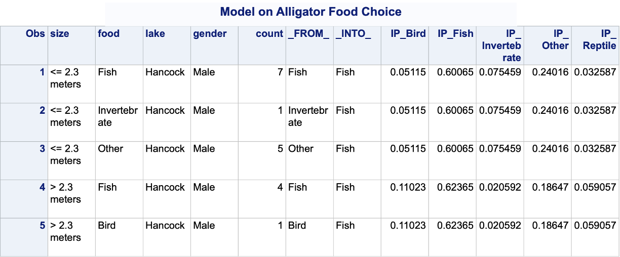{fig-align="center" width="6in"}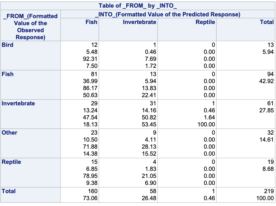{fig-align="center" width="6in"}The *IP* variables are the individual predicted probabilities for each of the categories of our target variable. Unlike binary logistic regression where we typically did not use a cut-off of 0.5 to determine which category we predict, in multinomial logistic regression we typically pick the category with the highest probability as our predicted category. The *FROM* and *INTO* variables are the actual target variable category and the predicted category for the target respectively.To see how the predicted categories compare with the actual target categories we can use PROC FREQ with a TABLES statement on the *FROM* and *INTO* variables.Accuracy is typically not as high in logistic regressions with more than two categories because there are more chances for incorrect predictions.:::


