Which variables should you drop from your model? This is a common question for all modeling, but especially logistic regression. In this section we will cover a popular variable selection technique - stepwise regression. This isn’t the only possible technique, but will be the primary focus here.
We will be going back to the Ames, Iowa dataset for exploring these techniques.
Stepwise regression techniques involve the three common methods:
Forward Selection
Backward Selection
Stepwise Selection
These techniques add or remove (depending on the technique) one variable at a time from your regression model to try and “improve” the model. There are a variety of different selection criteria to use to add or remove variables from a logistic regression. Two common approaches are to use either p-values or one of the pair of AIC/BIC.
Although p-values are falling out of popularity, it is primarily because people often use the 0.05 significance level without any regards to sample size. Although 0.05 is a good significance level for a sample size around 50, this level should be adjusted based on sample size.
However, it can be shown that mathematically the AIC/BIC criterion for adding or removing variables with stepwise selection (which is becoming very popular) is the same thing as using p-values in likelihood ratio tests. AIC is calculated as follows:
\[
AIC = -2 \log(L) + 2p
\] where \(L\) is the likelihood function and p is the number of variables being estimated in the model. Let’s compare two models - one with \(p\) variables and one with \(p+1\) variables. Assuming the additional variable lowers AIC, we can see the following relationship:
The right hand side of the equation is a Likelihood Ratio Test that follows a \(\chi^2_1\) distribution. So we know the significance level from this LRT is the following:
\[
1 - P(\chi^2_1 > 2) = 0.1573
\]
This means that the AIC selection method for stepwise selection is mathematically the same as a p-value stepwise selection technique with a significance level (\(\alpha\) level) of 0.1573 for continuous variables or binary categorical variables. More than two categories in a categorical variable would be greater than 1 degree of freedom in the calculation above.
The same math can be applied to the BIC selection technique as well. The BIC calculation is the following:
\[
BIC = -2 \log(L) + p \times \log(n)
\]
Working through the math, this is also a Likelihood Ratio Test that follows a \(\chi^2_1\) distribution. So we know the significance level from this LRT is the following:
\[
1 - P(\chi^2_1 > \log(n)) = \ldots
\]
Notice how the significance level changes depending on sample size due to the BIC equation, which is exactly what is recommended for any selection technique using p-values.
With that all understood, let’s look at the three common stepwise regression approaches.
Stepwise Selection
Here we will work through stepwise selection. In stepwise selection, the initial model is empty (contains no variables, only the intercept). Each variable is then tried to see if it is significant based on AIC/BIC or p-value with a specified significance level. The most significant variable (or the one that reduces the AIC/BIC the most) is then added to the model. Next, all variables in the model (here only one) are tested to see if they are still significant (or don’t hinder the AIC/BIC if dropped). If not, they are dropped. If so, then the remaining variables are again tested and the next most impactful variable (p-value or AIC/BIC depending on the approach) is added to the model. This process repeats until either no more significant variables are available to add or the same variable keeps being added and then removed from the model based on AIC/BIC or p-value (depending on the approach).
Let’s look at this approach using all of our softwares!
R’s step function traditionally uses either AIC or BIC for adding or removing variables from the stepwise regression techniques.
In R we must specify two models - the empty and full models - to step between. Notice the full model contains all the variables, while the empty model contains only the intercept (signified by ~ 1 in the formula). We then use the step function where we start at the empty model. The scope option tells R the lower (lower =) and upper (upper =) model to step between. The direction = "both" option tells R to use stepwise selection.
The model building summary is shown to have added variables based on lowest AIC. This may be different across different stepwise techniques.
At the time of writing this code deck, Python does not have nice capabilities to do this automatically in statsmodels, scikitlearn, or scipy. All resources found involve downloading and installing a package (mlxtend) that is not included by default in Anaconda or writing your own function. Scikit learn has something similar but uses the model’s coefficients to select, not p-values. This approach is completely unreasonable because coefficients reflect the units of the data. This means that smaller units in a variable lead to a smaller coefficient. The only way this would be appropriate is if all of the variables were standardized ahead of time. Scikitlearn has stepwise selection capabilities by evaluating a metric on cross-validation. However, cross-validation is not covered in this code deck. The corresponding Machine Learning code deck goes through this approach.
PROC LOGISTIC uses significance levels and p-values for adding or removing variables from the stepwise selection techniques. PROC LOGISTIC uses the selection = stepwise option to perform this technique. Notice also the slentry = and slstay = options where we specify the significance to both enter and stay in the model respectively. Here we chose 0.03 based on our sample size.
Code
ods html select ModelBuildingSummary ParameterEstimates ORPlot;proc logistic data=logistic.ames_train plots(only)=(oddsratio); class House_Style Full_Bath Half_Bath Central_Air / param=ref; model Bonus(event='1') = Gr_Liv_Area House_Style Garage_Area Fireplaces Full_Bath Half_Bath Lot_Area Central_Air Second_Flr_SF TotRms_AbvGrd First_Flr_SF / selection=stepwise slentry=0.005 slstay=0.005 clodds=pl clparm=pl; title 'Modeling Bonus Eligibility';run;quit;
The model building summary is shown to have added some variables. This may be different across different stepwise techniques.
Backward Selection
Here we will work through backward selection. In backward selection, the initial model is full (contains all variables, including the intercept). Each variable is then tried to see if it is significant based on AIC/BIC or p-value with a specified significance level. The least significant variable (or the one that hinders the AIC/BIC the most) is then dropped from the model. Then the remaining variables are again tested and the next least significant variable is dropped from the model. This process repeats until no more insignificant variables are available to drop or the AIC/BIC no longer improves with the deletion of another variable.
Let’s look at this approach using all of our softwares!
In R we must specify one model - the full model - to step backward from. Notice the full model contains all the variables. We then use the step function where we start at the full model. The direction = "backward" option tells R to use backward selection.
The model building summary is shown to have removed variables based on lowest AIC. This may be different across different stepwise techniques.
At the time of writing this code deck, Python does not have nice capabilities to do this automatically in statsmodels, scikitlearn, or scipy. All resources found involve downloading and installing a package (mlxtend) that is not included by default in Anaconda or writing your own function. Scikit learn has something similar but uses the model’s coefficients to select, not p-values. This approach is completely unreasonable because coefficients reflect the units of the data. This means that smaller units in a variable lead to a smaller coefficient. The only way this would be appropriate is if all of the variables were standardized ahead of time. Scikitlearn has backward selection capabilities by evaluating a metric on cross-validation. However, cross-validation is not covered in this code deck. The corresponding Machine Learning code deck goes through this approach.
PROC LOGISTIC uses the selection = backward option to perform this technique. Notice also the slstay = option where we specify the significance to stay in the model. Here we chose 0.03 based on our sample size.
Code
ods html select ModelBuildingSummary ParameterEstimates ORPlot;proc logistic data=logistic.ames_train plots(only)=(oddsratio); class House_Style Full_Bath Half_Bath Central_Air / param=ref; model Bonus(event='1') = Gr_Liv_Area House_Style Garage_Area Fireplaces Full_Bath Half_Bath Lot_Area Central_Air Second_Flr_SF TotRms_AbvGrd First_Flr_SF / selection=backward slstay=0.005 clodds=pl clparm=pl; title 'Modeling Bonus Eligibility';run;quit;
The model building summary is shown to have dropped some variables. This may be different across different stepwise techniques.
Forward with Interactions
Here we will work through forward selection. In forward selection, the initial model is empty (contains no variables, only the intercept). Each variable is then tried to see if it is significant based on AIC/BIC or p-value with a specified significance level. The most significant variable (or the one that reduces the AIC/BIC the most) is then added to the model. Then the remaining variables are again tested and the next most impactful variable (p-value or AIC/BIC depending on the approach) is added to the model. This process repeats until either no more significant variables are available to add to the model based on AIC/BIC or p-value (depending on the approach). This approach is the same as stepwise selection without the additional check at each step for possible removal.
Forward selection is the least used technique because stepwise selection does the same as forward selection with the added benefit of dropping insignificant variables. The main use for forward selection is to test higher order terms and interactions in models.
Let’s look at this approach using all of our softwares!
In R we must specify two models to step between. We then use the step function where we start at the empty model. The scope option tells R the lower (lower =) and upper (upper =) model to step between. The direction = "forward" option tells R to use stepwise selection.
Here we are testing some two-way interactions. This can be done in R by creating two models - the main effects model and the two-way interaction model. Here we set the starting point for forward selection at the main effects model and step up to the interaction model.
Notice that the modeling summary contains the addition of a couple of these interactions.
At the time of writing this code deck, Python does not have nice capabilities to do this automatically in statsmodels, scikitlearn, or scipy. All resources found involve downloading and installing a package (mlxtend) that is not included by default in Anaconda or writing your own function. Scikit learn has something similar but uses the model’s coefficients to select, not p-values. This approach is completely unreasonable because coefficients reflect the units of the data. This means that smaller units in a variable lead to a smaller coefficient. The only way this would be appropriate is if all of the variables were standardized ahead of time. Scikitlearn has forward selection capabilities by evaluating a metric on cross-validation. However, cross-validation is not covered in this code deck. The corresponding Machine Learning code deck goes through this approach.
PROC LOGISTIC uses the selection = forward option to perform this technique. Notice also the slentry = option where we specify the significance to enter in the model. Here we chose 0.03 based on our sample size.
This approach can be done in PROC LOGISTIC by placing a “|” in between variables. The “@2” is used to specify that we want only two-way interactions between these variables. The include = option forces SAS to include the first eleven variables - our main effects. This forces SAS to check all two-way interactions one at a time without having all of them in the model from the beginning like backward selection with interactions would do.
Here we can see that none of the interactions were added here.
Diagnostic Plots
Linear regression models contain residuals with properties that are very useful for model diagnostics. However, what is a residual in a logistic regression model? Since we don’t have actual probabilities to compare our predicted probabilities against, residuals are not as clearly defined. Instead we have pseudo “residuals” in logistic regression that we can explore further. Two examples of this are deviance residuals and Pearson residuals.
Deviance is a measure of how far a fitted model is from the fully saturated model. The fully saturated model is a model that predicts our data perfectly by essentially overfitting to it - a variable for each unique combination of inputs. This makes this model impractical for use, but good for comparison. The deviance is essentially our “error” from this “perfect” model. Logistic regression minimizes the sum of the squared deviances. Deviance residuals tell us how much each observation reduces the deviance.
Pearson residuals on the other hand tell us how much each observation changes the Pearson Chi-squared test for the overall model.
Other forms of measuring an observation’s influence on the logistic regression model are DFBetas and Cook’s D. Similar to their interpretation in linear regression, these two calculations tell us how each observation changes the estimation of each parameter individually (DFBeta) or how each observation changes the estimation of all the parameters holistically (Cook’s D).
Let’s see how to get all of these from our softwares!
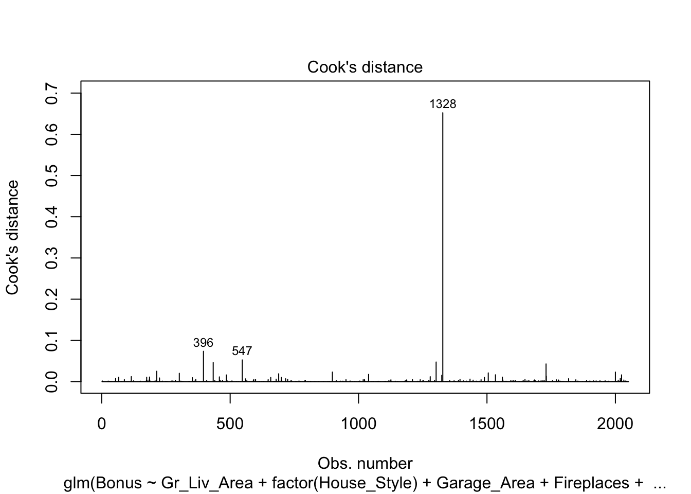
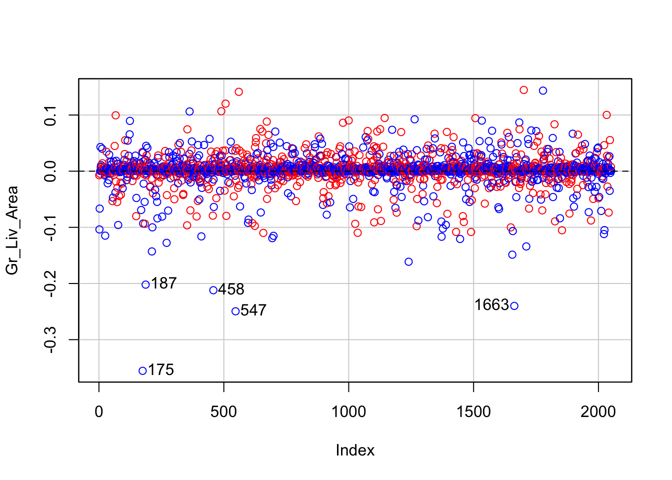
R has some wonderful diagnostics plots to show us these residuals. R also produces a list of these measures of influence as well as many more with the influence.measures function. Below only the first 6 observations are shown using the head function, but this is calculated for each of the observations. The 4th plot in the plot function on the logistic regression model object is the Cook’s D plot as shown below. The dfbetasPlots function produces the DFBetas plots, but only one is shown here.
The DFBetas plots show the standardized impact of each observation on the calculation of each of the parameters in the model. The main thing to look for in these plots are points that are far away from the rest of the observations.
These observations are not necessarily bad per se, but have a large influence on the model. These points might need to be investigated further to see if they are actually valid observations.
Python has some wonderful diagnostics plots to show us these residuals. Python also produces a list of these measures of influence as well as many more with the get_influence function. Below only the first 5 observations are shown using the head function, but this is calculated for each of the observations.
Here the plot_influence function shows the points graphed by their studentized residuals as well as their influence measured by H leverage - yet another way to measure impact on a regression model. At the time of writing this code deck, Python did not have an easy functionality for DFBetas plots.
Code
from matplotlib import pyplot as pltplt.cla()log_diag.plot_influence()plt.show()
SAS has some wonderful diagnostics plots to show us these residuals. In PROC LOGISTIC we ask for the influence and dfbetas plots from the plots = option.
Code
ods html select ParameterEstimates InfluencePlots DfBetasPlot;proc logistic data=logistic.ames_train plots(only label)=(influence dfbetas); class House_Style Full_Bath Half_Bath Central_Air / param=ref; model Bonus(event='1') = Gr_Liv_Area House_Style Garage_Area Fireplaces Full_Bath Lot_Area Central_Air TotRms_AbvGrd Gr_Liv_Area|Fireplaces @2/ clodds=pl clparm=pl; title 'Modeling Bonus Eligibility';run;quit;
The influence plots show a variety of plots. Among them are the Pearson residuals, Deviance residuals, and the difference in each of these for each observation. The main thing to look for in these plots are points that are far away from the rest of the observations.
The DFBetas plots show the standardized impact of each observation on the calculation of each of the parameters in the model. The main thing to look for in these plots are points that are far away from the rest of the observations.
These observations are not necessarily bad per se, but have a large influence on the model. These points might need to be investigated further to see if they are actually valid observations.
Calibration Curves
Another evaluation/diagnostic for logistic regression is the calibration curve. The calibration curve is a goodness-of-fit measure for logistic regression. Calibration measures how well predicted probabilities agree with actual frequency counts of outcomes (estimated linearly across the data set). These curves can help detect if predictions are consistently too high or low in your model.
If the curve is above the diagonal line, this indicates the model is predicting lower probabilities than actually observed. The opposite is true if the curve is below the diagonal line.
This is best used on larger samples since we are calculating the observed proportion of events in the data. In smaller samples this relationship is extrapolated out from the center and may not as accurately reflect the truth.
Let’s look at creating these in all of our softwares!
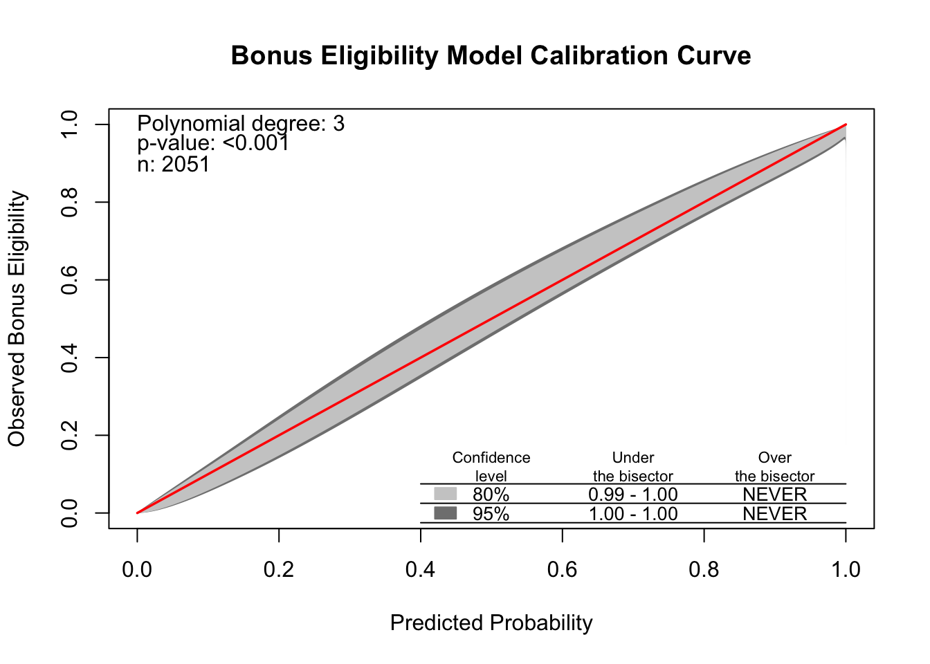
R produces a calibration curve using the givitiCalibrationBelt function. The inputs to this function are o = and e =. These are the observed target and expected target respectively. We place our actual target variable in the o = option and the predictions from our logistic regression model in the e = option. Since the model is being compared to training data the devel = internal option is specified. The maxDeg = option sets the maximum degree being tested for the curve.
library(givitiR)cali.curve <-givitiCalibrationBelt(o = train$Bonus,e =predict(logit.model, type ="response"),devel ="internal",maxDeg =5)plot(cali.curve, main ="Bonus Eligibility Model Calibration Curve",xlab ="Predicted Probability",ylab ="Observed Bonus Eligibility")
$m
[1] 3

$p.value
[1] 0
Since the diagonal line is contained in the confidence interval for our calibration curve, we do not notice any significant number of over or under predictions.
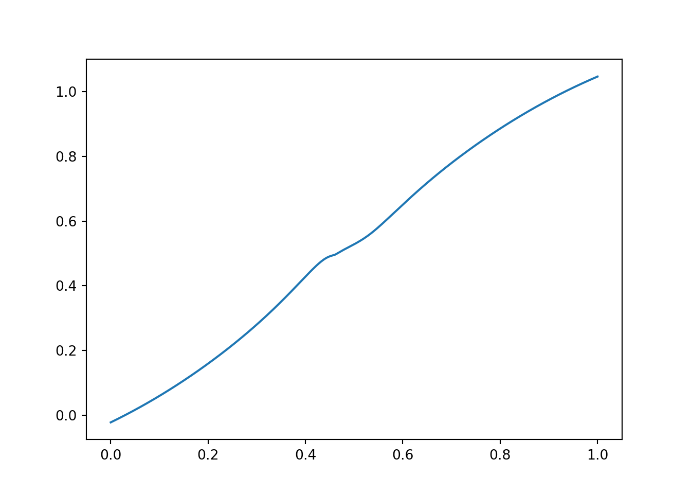
Python does not produce a calibration curve by default, but we can easily create it ourselves. After building the model with the GLM.from_forumla function and outputting the predicted probabilities from our training data using the predict function, we then sort these predicted probabilities using the sort_values function.
We then plot our our predicted probabilities. We then use the LOESS algorithm (using the statsmodels.api.nonparametric.lowess function) to fit a LOESS regression to our target variable (Bonus) using our predicted probabilities (Pred). We then plot this LOESS curve which is our calibration curve.
import numpy as npimport statsmodels.api as smtrain_sort = train.sort_values(by=['Pred'])smoothed = sm.nonparametric.lowess(exog=train_sort['Pred'], endog=train_sort['Bonus'], frac=0.85)plt.cla()plt.plot(smoothed[:, 0], smoothed[:, 1])plt.show()
Since the calibration curve estimation is relatively linear, we do not notice any significant number of over or under predictions.
SAS does not produce a calibration curve by default, but we can easily create it ourselves. After building the model with PROC LOGISTIC and outputting the predicted probabilities from our training data using the OUTPUT statement, we then sort these predicted probabilities using PROC SORT. We do this to easily plot the predicted probabilities in the SGPLOT procedure.
In PROC SGPLOT we use our predicted probabilities data set - here called cali. We then use the LOESS statement to fit a LOESS regression to our target variable (Bonus) using our predicted probabilities (PredProb). We allow for a cubic interpolation on this LOESS regression. The cml option produces a confidence interval around this curve. We then plot the diagonal line through the origin with a slope of 1. This produces our calibration curve.
Since the diagonal line is contained in the confidence interval for our calibration curve, we do not notice any significant number of over or under predictions.
Source Code
---title: "Subset Selection and Diagnostics"format: html: code-fold: show code-tools: trueeditor: visual---```{r}#| include: false#| warning: falselibrary(AmesHousing)ames <-make_ordinal_ames()library(tidyverse)ames <- ames %>%mutate(Bonus =ifelse(Sale_Price >175000, 1, 0))set.seed(123)ames <- ames %>%mutate(id =row_number())train <- ames %>%sample_frac(0.7)test <-anti_join(ames, train, by ='id')``````{python}#| include: falsetrain = r.traintest = r.test```# Stepwise RegressionWhich variables should you drop from your model? This is a common question for all modeling, but especially logistic regression. In this section we will cover a popular variable selection technique - stepwise regression. This isn't the only possible technique, but will be the primary focus here.We will be going back to the Ames, Iowa dataset for exploring these techniques.Stepwise regression techniques involve the three common methods:1. Forward Selection2. Backward Selection3. Stepwise SelectionThese techniques add or remove (depending on the technique) one variable at a time from your regression model to try and "improve" the model. There are a variety of different selection criteria to use to add or remove variables from a logistic regression. Two common approaches are to use either p-values or one of the pair of AIC/BIC.Although p-values are falling out of popularity, it is primarily because people often use the 0.05 significance level without any regards to sample size. Although 0.05 is a good significance level for a sample size around 50, this level should be adjusted based on sample size.However, it can be shown that mathematically the AIC/BIC criterion for adding or removing variables with stepwise selection (which is becoming very popular) is the same thing as using p-values in likelihood ratio tests. AIC is calculated as follows:$$AIC = -2 \log(L) + 2p$$ where $L$ is the likelihood function and p is the number of variables being estimated in the model. Let's compare two models - one with $p$ variables and one with $p+1$ variables. Assuming the additional variable lowers AIC, we can see the following relationship:```{=tex}\begin{aligned}AIC_{p+1} &< AIC_p \\-2 \log(L_{p+1}) + 2(p+1) &< -2 \log(L_p) + 2p \\2 &< 2(\log(L_{p+1}) - \log(L_p)) \\\end{aligned}```The right hand side of the equation is a Likelihood Ratio Test that follows a $\chi^2_1$ distribution. So we know the significance level from this LRT is the following:$$1 - P(\chi^2_1 > 2) = 0.1573$$This means that the AIC selection method for stepwise selection is mathematically the same as a p-value stepwise selection technique with a significance level ($\alpha$ level) of 0.1573 for continuous variables or binary categorical variables. More than two categories in a categorical variable would be greater than 1 degree of freedom in the calculation above.The same math can be applied to the BIC selection technique as well. The BIC calculation is the following:$$BIC = -2 \log(L) + p \times \log(n)$$Working through the math, this is also a Likelihood Ratio Test that follows a $\chi^2_1$ distribution. So we know the significance level from this LRT is the following:$$1 - P(\chi^2_1 > \log(n)) = \ldots$$Notice how the significance level changes depending on sample size due to the BIC equation, which is exactly what is recommended for any selection technique using p-values.With that all understood, let's look at the three common stepwise regression approaches.## Stepwise SelectionHere we will work through stepwise selection. In stepwise selection, the initial model is empty (contains no variables, only the intercept). Each variable is then tried to see if it is significant based on AIC/BIC or p-value with a specified significance level. The most significant variable (or the one that reduces the AIC/BIC the most) is then added to the model. Next, all variables in the model (here only one) are tested to see if they are still significant (or don't hinder the AIC/BIC if dropped). If not, they are dropped. If so, then the remaining variables are again tested and the next most impactful variable (p-value or AIC/BIC depending on the approach) is added to the model. This process repeats until either no more significant variables are available to add or the same variable keeps being added and then removed from the model based on AIC/BIC or p-value (depending on the approach).Let's look at this approach using all of our softwares!::: {.panel-tabset .nav-pills}## RR's `step` function traditionally uses either AIC or BIC for adding or removing variables from the stepwise regression techniques.In R we must specify two models - the empty and full models - to step between. Notice the full model contains all the variables, while the empty model contains only the intercept (signified by `~ 1` in the formula). We then use the `step` function where we start at the empty model. The `scope` option tells R the lower (`lower =`) and upper (`upper =`) model to step between. The `direction = "both"` option tells R to use stepwise selection.```{r}full.model <-glm(Bonus ~ Gr_Liv_Area +factor(House_Style) + Garage_Area + Fireplaces +factor(Full_Bath) +factor(Half_Bath) + Lot_Area +factor(Central_Air) + Second_Flr_SF + TotRms_AbvGrd + First_Flr_SF,data = train, family =binomial(link ="logit"))empty.model <-glm(Bonus ~1, data = train, family =binomial(link ="logit"))step.model <-step(empty.model,scope =list(lower=formula(empty.model),upper=formula(full.model)),direction ="both")summary(step.model)```The model building summary is shown to have added variables based on lowest AIC. This may be different across different stepwise techniques.## PythonAt the time of writing this code deck, Python does not have nice capabilities to do this automatically in statsmodels, scikitlearn, or scipy. All resources found involve downloading and installing a package (`mlxtend`) that is not included by default in Anaconda or writing your own function. Scikit learn has something similar but uses the model's coefficients to select, not p-values. This approach is completely unreasonable because coefficients reflect the units of the data. This means that smaller units in a variable lead to a smaller coefficient. The *only* way this would be appropriate is if all of the variables were standardized ahead of time. Scikitlearn has stepwise selection capabilities by evaluating a metric on cross-validation. However, cross-validation is *not* covered in this code deck. The corresponding Machine Learning code deck goes through this approach.## SASPROC LOGISTIC uses significance levels and p-values for adding or removing variables from the stepwise selection techniques. PROC LOGISTIC uses the `selection = stepwise` option to perform this technique. Notice also the `slentry =` and `slstay =` options where we specify the significance to both enter and stay in the model respectively. Here we chose 0.03 based on our sample size.```{r}#| eval: falseods html select ModelBuildingSummary ParameterEstimates ORPlot;proc logistic data=logistic.ames_train plots(only)=(oddsratio); class House_Style Full_Bath Half_Bath Central_Air / param=ref; model Bonus(event='1') = Gr_Liv_Area House_Style Garage_Area Fireplaces Full_Bath Half_Bath Lot_Area Central_Air Second_Flr_SF TotRms_AbvGrd First_Flr_SF / selection=stepwise slentry=0.005 slstay=0.005 clodds=pl clparm=pl; title 'Modeling Bonus Eligibility';run;quit;```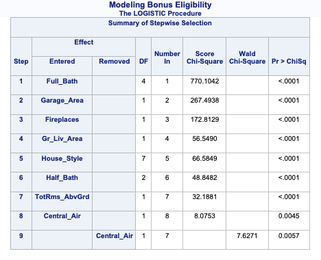{fig-align="center" width="6in"}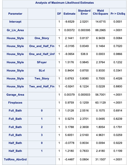{fig-align="center" width="6in"}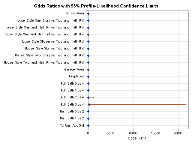{fig-align="center" width="6.67in"}The model building summary is shown to have added some variables. This may be different across different stepwise techniques.:::## Backward SelectionHere we will work through backward selection. In backward selection, the initial model is full (contains all variables, including the intercept). Each variable is then tried to see if it is significant based on AIC/BIC or p-value with a specified significance level. The least significant variable (or the one that hinders the AIC/BIC the most) is then dropped from the model. Then the remaining variables are again tested and the next least significant variable is dropped from the model. This process repeats until no more insignificant variables are available to drop or the AIC/BIC no longer improves with the deletion of another variable.Let's look at this approach using all of our softwares!::: {.panel-tabset .nav-pills}## RIn R we must specify one model - the full model - to step backward from. Notice the full model contains all the variables. We then use the `step` function where we start at the full model. The `direction = "backward"` option tells R to use backward selection.```{r}full.model <-glm(Bonus ~ Gr_Liv_Area +factor(House_Style) + Garage_Area + Fireplaces +factor(Full_Bath) +factor(Half_Bath) + Lot_Area +factor(Central_Air) + Second_Flr_SF + TotRms_AbvGrd + First_Flr_SF,data = train, family =binomial(link ="logit"))back.model <-step(full.model, direction ="backward")summary(back.model)```The model building summary is shown to have removed variables based on lowest AIC. This may be different across different stepwise techniques.## PythonAt the time of writing this code deck, Python does not have nice capabilities to do this automatically in statsmodels, scikitlearn, or scipy. All resources found involve downloading and installing a package (`mlxtend`) that is not included by default in Anaconda or writing your own function. Scikit learn has something similar but uses the model's coefficients to select, not p-values. This approach is completely unreasonable because coefficients reflect the units of the data. This means that smaller units in a variable lead to a smaller coefficient. The *only* way this would be appropriate is if all of the variables were standardized ahead of time. Scikitlearn has backward selection capabilities by evaluating a metric on cross-validation. However, cross-validation is *not* covered in this code deck. The corresponding Machine Learning code deck goes through this approach.## SASPROC LOGISTIC uses the `selection = backward` option to perform this technique. Notice also the `slstay =` option where we specify the significance to stay in the model. Here we chose 0.03 based on our sample size.```{r}#| eval: falseods html select ModelBuildingSummary ParameterEstimates ORPlot;proc logistic data=logistic.ames_train plots(only)=(oddsratio); class House_Style Full_Bath Half_Bath Central_Air / param=ref; model Bonus(event='1') = Gr_Liv_Area House_Style Garage_Area Fireplaces Full_Bath Half_Bath Lot_Area Central_Air Second_Flr_SF TotRms_AbvGrd First_Flr_SF / selection=backward slstay=0.005 clodds=pl clparm=pl; title 'Modeling Bonus Eligibility';run;quit;```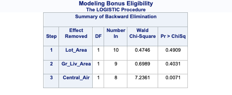{fig-align="center" width="6in"}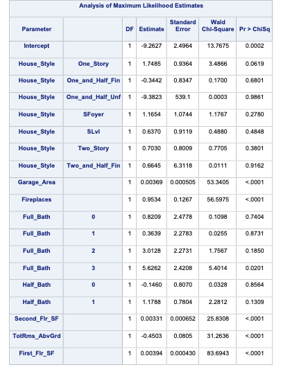{fig-align="center" width="6in"}The model building summary is shown to have dropped some variables. This may be different across different stepwise techniques.:::## Forward with InteractionsHere we will work through forward selection. In forward selection, the initial model is empty (contains no variables, only the intercept). Each variable is then tried to see if it is significant based on AIC/BIC or p-value with a specified significance level. The most significant variable (or the one that reduces the AIC/BIC the most) is then added to the model. Then the remaining variables are again tested and the next most impactful variable (p-value or AIC/BIC depending on the approach) is added to the model. This process repeats until either no more significant variables are available to add to the model based on AIC/BIC or p-value (depending on the approach). This approach is the same as stepwise selection without the additional check at each step for possible removal.Forward selection is the least used technique because stepwise selection does the same as forward selection with the added benefit of dropping insignificant variables. The main use for forward selection is to test higher order terms and interactions in models.Let's look at this approach using all of our softwares!::: {.panel-tabset .nav-pills}## RIn R we must specify two models to step between. We then use the `step` function where we start at the empty model. The `scope` option tells R the lower (`lower =`) and upper (`upper =`) model to step between. The `direction = "forward"` option tells R to use stepwise selection.Here we are testing some two-way interactions. This can be done in R by creating two models - the main effects model and the two-way interaction model. Here we set the starting point for forward selection at the main effects model and step up to the interaction model.```{r}#| warning: falsemain.model <-glm(Bonus ~ Gr_Liv_Area +factor(House_Style) + Garage_Area +factor(Fireplaces) +factor(Full_Bath) +factor(Half_Bath) + Lot_Area +factor(Central_Air) + Second_Flr_SF + TotRms_AbvGrd + First_Flr_SF,data = train, family =binomial(link ="logit"))int.model <-glm(Bonus ~ Gr_Liv_Area +factor(House_Style) + Garage_Area + Fireplaces +factor(Full_Bath) +factor(Half_Bath) + Lot_Area +factor(Central_Air) + Second_Flr_SF + TotRms_AbvGrd + First_Flr_SF + Gr_Liv_Area*factor(House_Style) + TotRms_AbvGrd*factor(House_Style) + Gr_Liv_Area*factor(Fireplaces),data = train, family =binomial(link ="logit"))for.model <-step(main.model,scope =list(lower=formula(main.model),upper=formula(int.model)),direction ="forward")summary(for.model)```Notice that the modeling summary contains the addition of a couple of these interactions.## PythonAt the time of writing this code deck, Python does not have nice capabilities to do this automatically in statsmodels, scikitlearn, or scipy. All resources found involve downloading and installing a package (`mlxtend`) that is not included by default in Anaconda or writing your own function. Scikit learn has something similar but uses the model's coefficients to select, not p-values. This approach is completely unreasonable because coefficients reflect the units of the data. This means that smaller units in a variable lead to a smaller coefficient. The *only* way this would be appropriate is if all of the variables were standardized ahead of time. Scikitlearn has forward selection capabilities by evaluating a metric on cross-validation. However, cross-validation is *not* covered in this code deck. The corresponding Machine Learning code deck goes through this approach.## SASPROC LOGISTIC uses the `selection = forward` option to perform this technique. Notice also the `slentry =` option where we specify the significance to enter in the model. Here we chose 0.03 based on our sample size.This approach can be done in PROC LOGISTIC by placing a "\|" in between variables. The "@2" is used to specify that we want only two-way interactions between these variables. The `include =` option forces SAS to include the first eleven variables - our main effects. This forces SAS to check all two-way interactions one at a time without having all of them in the model from the beginning like backward selection with interactions would do.```{r}#| eval: falseods html select ModelBuildingSummary ParameterEstimates ORPlot;proc logistic data=logistic.ames_train plots(only)=(oddsratio); class House_Style Full_Bath Half_Bath Central_Air / param=ref; model Bonus(event='1') = Gr_Liv_Area House_Style Garage_Area Fireplaces Full_Bath Half_Bath Lot_Area Central_Air Second_Flr_SF TotRms_AbvGrd First_Flr_SF Gr_Liv_Area|House_Style|Fireplaces @2/ selection=forward slentry=0.05 clodds=pl clparm=pl include=11; title 'Modeling Bonus Eligibility';run;quit;```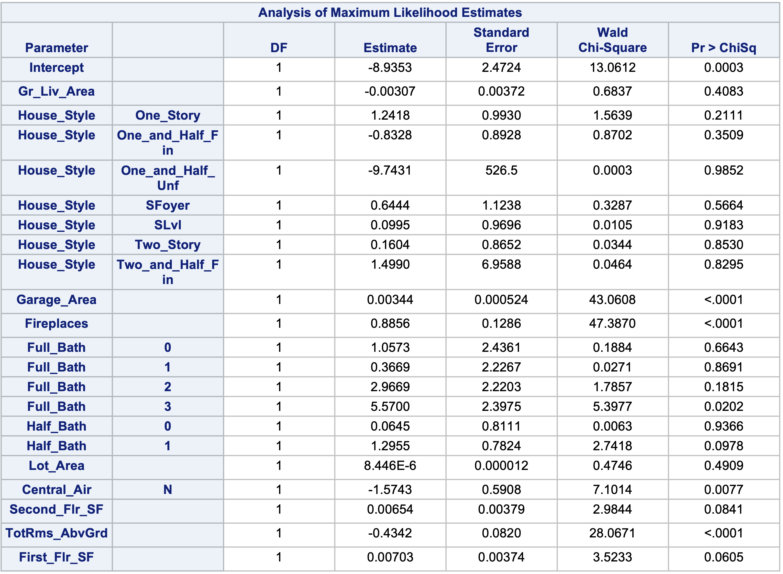{fig-align="center" width="6in"}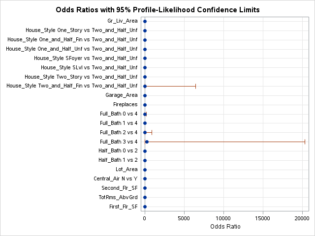{fig-align="center"}Here we can see that none of the interactions were added here.:::# Diagnostic PlotsLinear regression models contain residuals with properties that are very useful for model diagnostics. However, what is a residual in a logistic regression model? Since we don't have actual probabilities to compare our predicted probabilities against, residuals are not as clearly defined. Instead we have pseudo "residuals" in logistic regression that we can explore further. Two examples of this are **deviance residuals** and **Pearson residuals**.Deviance is a measure of how far a fitted model is from the fully saturated model. The fully saturated model is a model that predicts our data perfectly by essentially overfitting to it - a variable for each unique combination of inputs. This makes this model impractical for use, but good for comparison. The deviance is essentially our "error" from this "perfect" model. Logistic regression minimizes the sum of the squared deviances. Deviance residuals tell us how much each observation reduces the deviance.Pearson residuals on the other hand tell us how much each observation changes the Pearson Chi-squared test for the overall model.Other forms of measuring an observation's influence on the logistic regression model are **DFBetas** and **Cook's D**. Similar to their interpretation in linear regression, these two calculations tell us how each observation changes the estimation of each parameter individually (DFBeta) or how each observation changes the estimation of all the parameters holistically (Cook's D).Let's see how to get all of these from our softwares!::: {.panel-tabset .nav-pills}## RR has some wonderful diagnostics plots to show us these residuals. R also produces a list of these measures of influence as well as many more with the `influence.measures` function. Below only the first 6 observations are shown using the `head` function, but this is calculated for each of the observations. The 4th plot in the `plot` function on the logistic regression model object is the Cook's D plot as shown below. The `dfbetasPlots` function produces the DFBetas plots, but only one is shown here.```{r}#| message: falselogit.model <-glm(Bonus ~ Gr_Liv_Area +factor(House_Style) + Garage_Area + Fireplaces +factor(Full_Bath) + Lot_Area +factor(Central_Air) + TotRms_AbvGrd + Gr_Liv_Area:Fireplaces,data = train, family =binomial(link ="logit"))summary(logit.model)library(car)head(influence.measures(logit.model)$infmat)plot(logit.model, 4)dfbetasPlots(logit.model, terms ="Gr_Liv_Area", id.n =5,col =ifelse(logit.model$y ==1, "red", "blue"))```The DFBetas plots show the standardized impact of each observation on the calculation of each of the parameters in the model. The main thing to look for in these plots are points that are far away from the rest of the observations.These observations are not necessarily bad per se, but have a large influence on the model. These points might need to be investigated further to see if they are actually valid observations.## PythonPython has some wonderful diagnostics plots to show us these residuals. Python also produces a list of these measures of influence as well as many more with the `get_influence` function. Below only the first 5 observations are shown using the `head` function, but this is calculated for each of the observations.```{python}from statsmodels.genmod.families import Binomialfrom statsmodels.genmod.generalized_linear_model import GLMlog_model = GLM.from_formula('Bonus ~ Gr_Liv_Area + Garage_Area + Fireplaces + C(Full_Bath) + Lot_Area + C(Central_Air) + TotRms_AbvGrd + Gr_Liv_Area:Fireplaces', data = train, family = Binomial()).fit()log_model.summary()``````{python}import statsmodels.stats.tests.test_influencelog_diag = log_model.get_influence()log_diag.summary_frame().head()```Here the `plot_influence` function shows the points graphed by their studentized residuals as well as their influence measured by H leverage - yet another way to measure impact on a regression model. At the time of writing this code deck, Python did not have an easy functionality for DFBetas plots.```{python}from matplotlib import pyplot as pltplt.cla()log_diag.plot_influence()plt.show()```## SASSAS has some wonderful diagnostics plots to show us these residuals. In PROC LOGISTIC we ask for the `influence` and `dfbetas` plots from the `plots =` option.```{r}#| eval: falseods html select ParameterEstimates InfluencePlots DfBetasPlot;proc logistic data=logistic.ames_train plots(only label)=(influence dfbetas); class House_Style Full_Bath Half_Bath Central_Air / param=ref; model Bonus(event='1') = Gr_Liv_Area House_Style Garage_Area Fireplaces Full_Bath Lot_Area Central_Air TotRms_AbvGrd Gr_Liv_Area|Fireplaces @2/ clodds=pl clparm=pl; title 'Modeling Bonus Eligibility';run;quit;```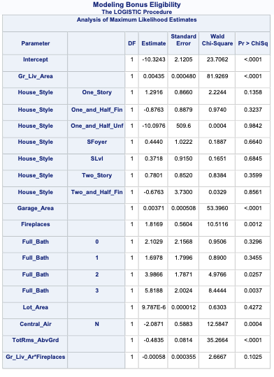{fig-align="center" width="6in"}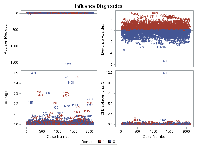{fig-align="center"}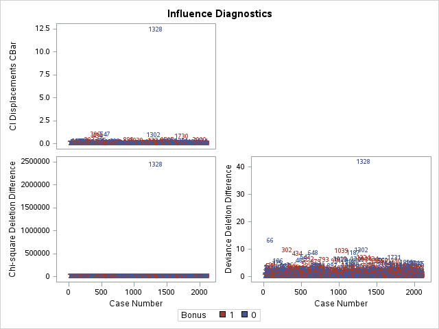{fig-align="center"}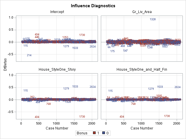{fig-align="center"}The influence plots show a variety of plots. Among them are the Pearson residuals, Deviance residuals, and the difference in each of these for each observation. The main thing to look for in these plots are points that are far away from the rest of the observations.The DFBetas plots show the standardized impact of each observation on the calculation of each of the parameters in the model. The main thing to look for in these plots are points that are far away from the rest of the observations.These observations are not necessarily bad per se, but have a large influence on the model. These points might need to be investigated further to see if they are actually valid observations.:::# Calibration CurvesAnother evaluation/diagnostic for logistic regression is the **calibration curve**. The calibration curve is a goodness-of-fit measure for logistic regression. Calibration measures how well predicted probabilities agree with actual frequency counts of outcomes (estimated linearly across the data set). These curves can help detect if predictions are consistently too high or low in your model.If the curve is above the diagonal line, this indicates the model is predicting **lower** probabilities than actually observed. The opposite is true if the curve is below the diagonal line.This is best used on larger samples since we are calculating the observed proportion of events in the data. In smaller samples this relationship is extrapolated out from the center and may not as accurately reflect the truth.Let's look at creating these in all of our softwares!::: {.panel-tabset .nav-pills}## RR produces a calibration curve using the `givitiCalibrationBelt` function. The inputs to this function are `o =` and `e =`. These are the observed target and expected target respectively. We place our actual target variable in the `o =` option and the predictions from our logistic regression model in the `e =` option. Since the model is being compared to training data the `devel = internal` option is specified. The `maxDeg =` option sets the maximum degree being tested for the curve.```{r}#| message: falselogit.model <-glm(Bonus ~ Gr_Liv_Area +factor(House_Style) + Garage_Area + Fireplaces +factor(Full_Bath) + Lot_Area +factor(Central_Air) + TotRms_AbvGrd + Gr_Liv_Area:Fireplaces,data = train, family =binomial(link ="logit"))summary(logit.model)library(givitiR)cali.curve <-givitiCalibrationBelt(o = train$Bonus,e =predict(logit.model, type ="response"),devel ="internal",maxDeg =5)plot(cali.curve, main ="Bonus Eligibility Model Calibration Curve",xlab ="Predicted Probability",ylab ="Observed Bonus Eligibility")```Since the diagonal line is contained in the confidence interval for our calibration curve, we do not notice any significant number of over or under predictions.## PythonPython does not produce a calibration curve by default, but we can easily create it ourselves. After building the model with the `GLM.from_forumla` function and outputting the predicted probabilities from our training data using the `predict` function, we then sort these predicted probabilities using the `sort_values` function.We then plot our our predicted probabilities. We then use the LOESS algorithm (using the `statsmodels.api.nonparametric.lowess` function) to fit a LOESS regression to our target variable (*Bonus*) using our predicted probabilities (*Pred*). We then plot this LOESS curve which is our calibration curve.```{python}log_model = GLM.from_formula('Bonus ~ Gr_Liv_Area + C(House_Style) + Garage_Area + Fireplaces + C(Full_Bath) + Lot_Area + C(Central_Air) + TotRms_AbvGrd + Gr_Liv_Area:Fireplaces', data = train, family = Binomial()).fit()log_model.summary()train['Pred'] = log_model.predict(train)``````{python}import numpy as npimport statsmodels.api as smtrain_sort = train.sort_values(by=['Pred'])smoothed = sm.nonparametric.lowess(exog=train_sort['Pred'], endog=train_sort['Bonus'], frac=0.85)plt.cla()plt.plot(smoothed[:, 0], smoothed[:, 1])plt.show()```Since the calibration curve estimation is relatively linear, we do not notice any significant number of over or under predictions.## SASSAS does not produce a calibration curve by default, but we can easily create it ourselves. After building the model with PROC LOGISTIC and outputting the predicted probabilities from our training data using the OUTPUT statement, we then sort these predicted probabilities using PROC SORT. We do this to easily plot the predicted probabilities in the SGPLOT procedure.In PROC SGPLOT we use our predicted probabilities data set - here called *cali*. We then use the LOESS statement to fit a LOESS regression to our target variable (*Bonus*) using our predicted probabilities (*PredProb*). We allow for a cubic interpolation on this LOESS regression. The `cml` option produces a confidence interval around this curve. We then plot the diagonal line through the origin with a slope of 1. This produces our calibration curve.```{r}#| eval: falseproc logistic data=logistic.ames_train noprint; class House_Style Full_Bath Half_Bath Central_Air / param=ref; model Bonus(event='1') = Gr_Liv_Area House_Style Garage_Area Fireplaces Full_Bath Lot_Area Central_Air TotRms_AbvGrd Gr_Liv_Area|Fireplaces @2/ clodds=pl clparm=pl; output out=cali predicted=PredProb;run;proc sort data=cali; by PredProb;run;proc sgplot data=cali noautolegend aspect=1; loess x=PredProb y=Bonus / interpolation=cubic clm; lineparm x=0 y=0 slope=1/ lineattrs=(color=grey pattern=dash); title 'Calibration Curve for Bonus Eligibility Data';run;```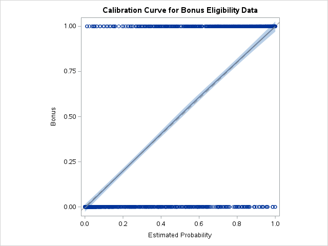{fig-align="center"}Since the diagonal line is contained in the confidence interval for our calibration curve, we do not notice any significant number of over or under predictions.:::