Code
table(churn$churn)
FALSE  TRUE
 2850   154
Code
prop.table(table(churn$churn))
     FALSE       TRUE
0.94873502 0.05126498
Code
churn$id <- 1:length(churn$churn)There are a lot of considerations one should take with data involving a logistic regression. What happens if my event of interest is a rare occurrence in my data set? How do categorical variables influence the convergence of my logistic regression model? These are the important things we need to account for in modeling.
Classification models try to predict categorical target variables, typically where one of the categories is of main interest. What if this category of interest doesn’t happen frequently in the data set? This is referred to as rare-event modeling and exists in many fields such as fraud, credit default, marketing responses, and rare weather events. The typical cut-off people use to decide if their event is rare is 5%. If your event occurs less than 5% of the time, you should adjust your modeling to account for this.
We will be using the telecomm data set data set to model the association between various factors and a customer churning from the company. The variables in the data set are the following:
| Variable | Description |
|---|---|
| account_length | length of time with company |
| international_plan | yes, no |
| voice_mail_plan | yes, no |
| customer_service_calls | number of service calls |
| total_day_minutes | minutes used during daytime |
| total_day_calls | calls used during daytime |
| total_day_charge | cost of usage during daytime |
| Same as previous 3 for evening, night, international | same as above |
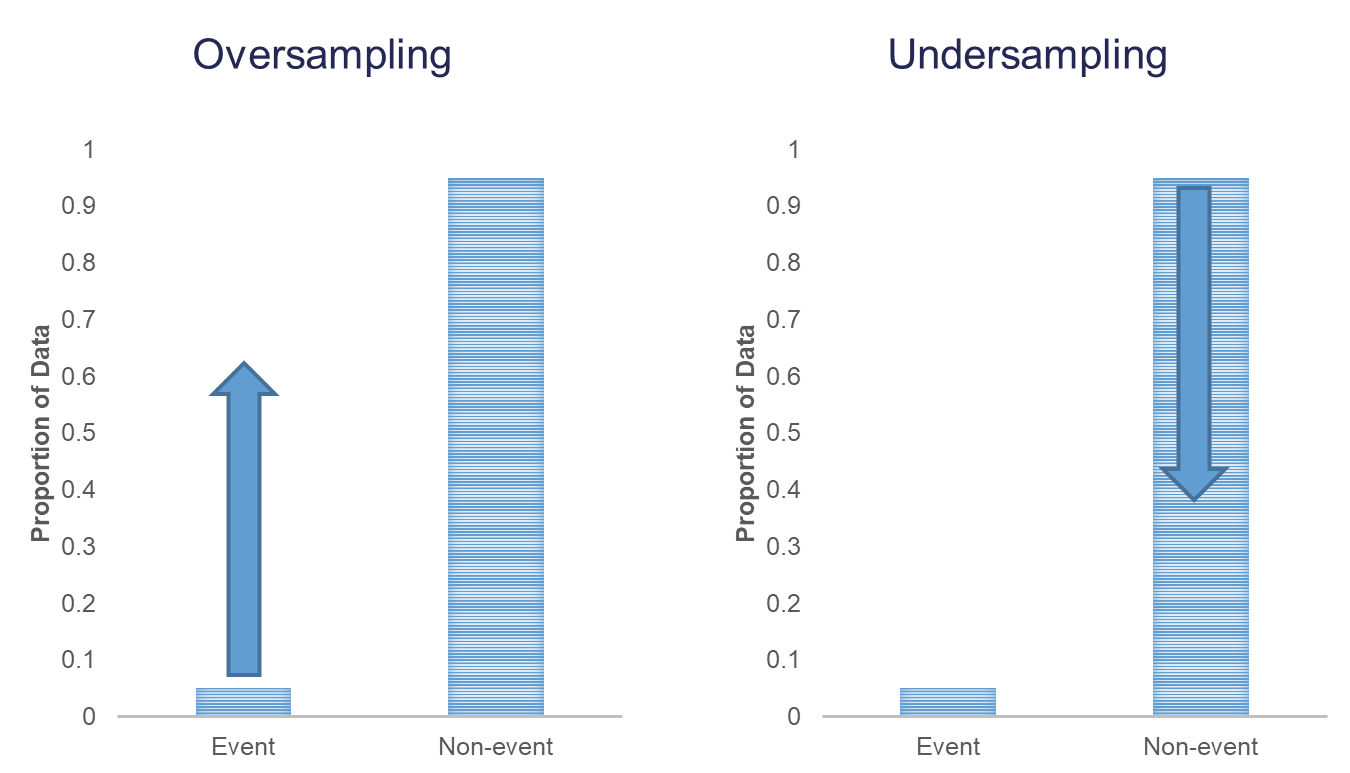
When you have a rare event situation, you can adjust for this by balancing out the sample in your training data set. This can be done through sampling techniques typically called oversampling. When oversampling, you can either over or under sample your target variable to get balance.
Oversampling is when you replicate your rare event enough times to balance out with your non-events in your training data sets. There are a variety of different ways to replicate observations, but for now we will only focus on true replication - copying our actual observations at random until we get balance. This will inflate our training data set size.
Undersampling is when we randomly sample from the non-events in our training data set only enough observations to balance out with events. This will make our training data set size much smaller. These are both represented in the following figure:
Let’s see how to perform these in each of our softwares!
In R we can easily perform both over and under sampling respectively. First, we examine the proportional breakdown of our target variable with the table and prop.table functions. Specifically we want to view the churn variable. We can see below that we have roughly 5% of the customers in our data churn from the company. We also create a new id variable in the dataset by simply starting with the number 1 and going through the length of the dataset.
table(churn$churn)
FALSE TRUE
2850 154 prop.table(table(churn$churn))
FALSE TRUE
0.94873502 0.05126498 churn$id <- 1:length(churn$churn)It is easy to perform undersampling in R with some basic data manipulation functions. Below we use the group_by function to group by our target variable churn. From the above output, we have 154 churners in our dataset. Let’s sample 104 of them for the training and leave the remaining 50 for testing. Now we just need a random sample of 104 of each of the churners and non-churners from our dataset. For this we use the sample_n function. The training data is defined as the rows that have these row ID’s and the test data set is defined as the rows that don’t have these ID’s. The table functions then show the number of observations in each data set for the churn variable.
library(tidyverse)

set.seed(12345)
train_u <- churn %>%
  group_by(churn) %>%
  sample_n(104)

test_u <- churn[-train_u$id,]

table(train_u$churn)
FALSE  TRUE
104 104 table(test_u$churn)
FALSE  TRUE
 2746    50
Oversampling is also easy to perform in R. There are many ways to duplicate rows in R. First, we use the sample_frac function to isolate down to 70% of the observations. From there we want to isolate the churners to replicate them. For this we use the filter function with churn equal to TRUE. Next, we use the slice and rep functions to repeat each of the observations 10 times (set by the each = option). Lastly, we want to isolate the non-churners, again with the filter function to blend these two sets together. With the rbind function we combine our non-churners and the replicated churners together.
set.seed(12345)
train_o <- churn %>%
  sample_frac(0.70)

train_o_T <- train_o %>%
  filter(churn == TRUE) %>%
  slice(rep(1:n(), each = 10))

train_o_F <- train_o %>%
  filter(churn == FALSE)

train_o <- rbind(train_o_F, train_o_T)

test_o <- churn[-train_o$id,]

table(train_o$churn)
FALSE  TRUE
1996 1070 table(test_o$churn)
FALSE  TRUE
  854    47
In Python we can easily perform both over and under sampling respectively. First, we examine the proportional breakdown of our target variable with the crosstab function divided by the sum of the rows in the table to get the proportions. Specifically we want to view the churn variable. We can see below that we have roughly 5% of the customers in our data churn from the company.
pd.crosstab(index = churn['churn'], columns = "prop")/pd.crosstab(index = churn['churn'], columns = "prop").sum()col_0 prop
churn
False 0.948735
True 0.051265We also create a new id variable in the dataset by simply starting with the number 1 and going through the length of the dataset. It is easy to perform undersampling in Python with some basic data manipulation functions. Below we use the groupby function to group by our target variable churn. From the above output, we have 154 churners in our dataset. Let’s sample 104 of them for the training and leave the remaining 50 for testing. Now we just need a random sample of 104 of each of the churners and non-churners from our dataset. For this we use the sample function. The training data is defined as the rows that have these row ID’s and the test data set is defined as the rows that don’t have these ID’s.
churn['id'] = churn.index + 1

train_u = churn.groupby("churn").sample(n = 104, random_state = 1234)

test_u = churn[~churn['id'].isin(train_u['id'])]
The crosstab functions then show the number of observations in each data set for the churn variable.
pd.crosstab(index = train_u['churn'], columns = "count")col_0 count
churn
False 104
True 104pd.crosstab(index = test_u['churn'], columns = "count")col_0 count
churn
False 2746
True 50Oversampling is also easy to perform in Python. There are many ways to duplicate rows in Python. First, we use the sample function with the frac option to isolate down to 70% of the observations. From there we want to isolate the churners to replicate them. For this we create a new dataframe, is_churn, with churn equal to True. Next, we use the concat function to repeat each of the observations repeating this process 9 times.
train_churn = churn.sample(frac = 0.7)

is_churn = train_churn['churn'] == True

concat_list = [
  train_churn,
  train_churn[is_churn],
  train_churn[is_churn],
  train_churn[is_churn],
  train_churn[is_churn],
  train_churn[is_churn],
  train_churn[is_churn],
  train_churn[is_churn],
  train_churn[is_churn],
  train_churn[is_churn]
]

train_o = pd.concat(concat_list, ignore_index = True)

test_o = churn[~churn['id'].isin(train_o['id'])]

pd.crosstab(index = train_o['churn'], columns = "count")
col_0 count
churn
False 1994
True 1090pd.crosstab(index = test_o['churn'], columns = "count")col_0 count
churn
False 856
True 45We now have an undersampled data set to build models on. There are two typical ways to adjust models from over or undersampling - adjusting the intercept and weighting.
Let’s examine this data set and how we can adjust our models accordingly with each technique.
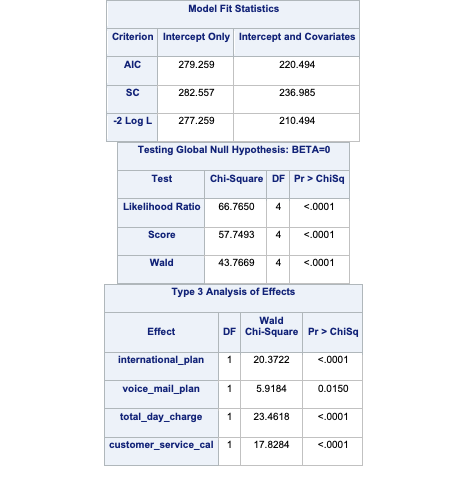
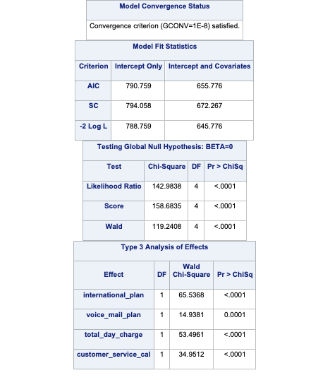
In SAS it is rather easy to replicate observations with the DATA STEP so we will not cover oversampling here. However, randomly undersampling isn’t as trivial. First, we examine the proportional breakdown of our target variable with PROC FREQ. Specifically we want to view the churn variable. We can see below that we have roughly 5% of the customers in our data churn. With PROC SURVERYSELECT we have a few important options. The data = option inputs our data set of interest - here the whole data set. The out = option specifies the data set name that will contain the observations we sampled. The seed = option is important to specify so we can replicate the results and get the same sample repeatedly. The sampsize = option specifies how many observations we want in our undersampled data for each category (event and nonevent). Here we want 100 in each, making our training data set 200 observations with a 50/50 balance of event to non-event observations. We don’t want to use all the event observations in the training set so we can have some still in the testing data set. The outall option is very important. It will keep all the observations from our original data set (from the data = option) in the new data set (from the out = option) with a new variable added to flag which observations have been sampled and which have not. Without this option we would only have the sampled observations in this new data set. Lastly, the STRATA statement specifies the variable we want to stratify our sample on - here the target variable.
proc freq data=logistic.tele_churn;
   table churn;
run;

proc surveyselect data = logistic.tele_churn noprint out=churn_over seed=12345
                  sampsize=(100 100) outall;
   strata churn;
run;

proc freq data=churn_over;
   table churn*selected / norow nopercent;
run;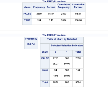
After running the PROC SURVERYSELECT, we can see from the PROC FREQ that we have a new variable called Selected in our data set. There are 200 observations with a value for 1 for Selected (our sampled observations) with a balance of 100 events and 100 non-events. The remaining observations have a value of 0 for the Selected variable. We will use the DATA STEP to split these selected and non-selected observations into our training and validation data set respectively.
data churn_t churn_v;
   set churn_over;
   if selected = 1 then output churn_t;
   else output churn_v;
run;
We now have an undersampled data set to build models on. There are two typical ways to adjust models from over or undersampling - adjusting the intercept and weighting.
Let’s examine this data set and how we can adjust our models accordingly with each technique.
One of the ways of adjusting your logistic regression model to account for the sampling to balance the events with non-events is by adjusting the intercept from the logistic regression model. The intercept is what sets the “baseline” probability in your model which is now too high. You can adjust your predicted probabilities from the regression model to account for this incorrect intercept. They can be adjusted with the following equation:
\[ \hat{p}_i = \frac{\hat{p}_i^* \rho_0 \pi_1}{(1-\hat{p}_i^*)\rho_1\pi_0 + \hat{p}_i^* \rho_0 \pi_1}\]
where \(\hat{p}_i^*\) is the unadjusted predicted probability, \(\pi_1\) and \(\pi_0\) are the population proportions of your target variable categories (1 and 0), and \(\rho_1\) and \(\rho_0\) are the sample proportions of your target variable categories (1 and 0).
Let’s see how to do this in each of our softwares!
Luckily, this is rather easy to do in R as we can directly adjust the predicted probability vector with this equation. First, we build a logistic regression model as seen in the previous section using the glm function on our undersampled training data. We can use the predict function to obtain our predicted probabilities from this model. These are biased probabilities however because of our sampling. By simply applying the equation above on the predicted probability vector we can get unbiased predicted probabilities.
logit.model <- glm(churn ~ factor(international_plan) +
                           factor(voice_mail_plan) +
                           total_day_charge +
                           customer_service_calls,
                   data = train_u, family = binomial(link = "logit"))
summary(logit.model)
Call:
glm(formula = churn ~ factor(international_plan) + factor(voice_mail_plan) +
    total_day_charge + customer_service_calls, family = binomial(link = "logit"),
    data = train_u)

Coefficients:
                              Estimate Std. Error z value Pr(>|z|)
(Intercept)                   -5.81880    0.95939  -6.065 1.32e-09 ***
factor(international_plan)yes  2.97995    0.57057   5.223 1.76e-07 ***
factor(voice_mail_plan)yes    -0.85107    0.41372  -2.057   0.0397 *
total_day_charge               0.12898    0.02234   5.773 7.79e-09 ***
customer_service_calls         0.78520    0.14947   5.253 1.50e-07 ***
---
Signif. codes:  0 '***' 0.001 '**' 0.01 '*' 0.05 '.' 0.1 ' ' 1

(Dispersion parameter for binomial family taken to be 1)

    Null deviance: 288.35  on 207  degrees of freedom
Residual deviance: 195.24  on 203  degrees of freedom
AIC: 205.24

Number of Fisher Scoring iterations: 5test_u_p_bias <- predict(logit.model, newdata = test_u, type = "response")
test_u_p <- (test_u_p_bias*(104/208)*(154/3004))/((1-test_u_p_bias)*(104/208)*(2850/3004)+test_u_p_bias*(104/208)*(154/3004))
test_u <- data.frame(test_u, 'Pred' = test_u_p)
head(test_u_p) 1 2 3 4 5 6
0.04788873 0.00516951 0.03230002 0.91516214 0.56312205 0.29766875 We then store these as a new column in our test data set.
Luckily, this is rather easy to do in Python as we can directly adjust the predicted probability vector with this equation. First, we build a logistic regression model as seen in the previous section using the GLM.from_formula function on our undersampled training data.
from statsmodels.genmod.families import Binomial
from statsmodels.genmod.generalized_linear_model import GLM

train_u.churn = train_u.churn.replace({True: 1, False: 0})
<string>:2: FutureWarning: Downcasting behavior in `replace` is deprecated and will be removed in a future version. To retain the old behavior, explicitly call `result.infer_objects(copy=False)`. To opt-in to the future behavior, set `pd.set_option('future.no_silent_downcasting', True)`log_model = GLM.from_formula('churn ~ C(international_plan) + C(voice_mail_plan) + total_day_charge + customer_service_calls', data = train_u, family = Binomial()).fit()
log_model.summary()| Dep. Variable: | churn | No. Observations: | 208 |
| Model: | GLM | Df Residuals: | 203 |
| Model Family: | Binomial | Df Model: | 4 |
| Link Function: | Logit | Scale: | 1.0000 |
| Method: | IRLS | Log-Likelihood: | -109.63 |
| Date: | Mon, 24 Jun 2024 | Deviance: | 219.26 |
| Time: | 19:32:51 | Pearson chi2: | 220. |
| No. Iterations: | 5 | Pseudo R-squ. (CS): | 0.2826 |
| Covariance Type: | nonrobust |
| coef | std err | z | P>|z| | [0.025 | 0.975] | |
| Intercept | -4.3060 | 0.733 | -5.873 | 0.000 | -5.743 | -2.869 |
| C(international_plan)[T.yes] | 2.3759 | 0.518 | 4.583 | 0.000 | 1.360 | 3.392 |
| C(voice_mail_plan)[T.yes] | -0.6272 | 0.420 | -1.493 | 0.135 | -1.451 | 0.196 |
| total_day_charge | 0.0921 | 0.018 | 5.228 | 0.000 | 0.058 | 0.127 |
| customer_service_calls | 0.5964 | 0.121 | 4.935 | 0.000 | 0.360 | 0.833 |
We can use the predict function to obtain our predicted probabilities from this model. These are biased probabilities however because of our sampling. By simply applying the equation above on the predicted probability vector we can get unbiased predicted probabilities.
test_u['pred_bias'] = log_model.predict(test_u)

test_u['pred'] = (test_u['pred_bias']*(104/208)*(154/3004))/((1 - test_u['pred_bias'])*(104/208)*(2850/3004) + test_u['pred_bias']*(104/208)*(154/3004))

test_u['pred'].head()
0 0.042905
1 0.008788
2 0.031863
3 0.737190
4 0.389486
Name: pred, dtype: float64We then store these as a new column in our test data set.
Luckily SAS will do this for us! All we have to do is give SAS the prior proportions from our population. In PROC FREQ we are again looking at the original distribution of the churn variable, but this time recording the proportions of 1’s and 0’s. The out = option saves the frequency analysis to a data set here called priors. In this data set we drop the percent variable with the drop = option and rename the count variable to prior with the rename = option.
From there we build our logistic regression in PROC LOGISTIC as we have previously learned in earlier sections. The main difference comes in the SCORE statement. The data = option specifies the data set we want to score (here the validation data set) and the out = option specifies the name of our newly scored data set. The prior = option specifies the name of the data set that contains the prior proportions for the target variable (the priors data set we created from PROC FREQ).
proc freq data=logistic.tele_churn noprint;
   table churn / out=priors(drop=percent rename=(count=_prior_));
run;

proc logistic data=churn_t;
   class international_plan(ref='no') voice_mail_plan(ref='no') / param=ref;
   model churn(event='TRUE') = international_plan
                               voice_mail_plan
                               total_day_charge
                               customer_service_calls / clodds=pl;
   score data=churn_v prior=priors out=churn_scored1;
run;
quit;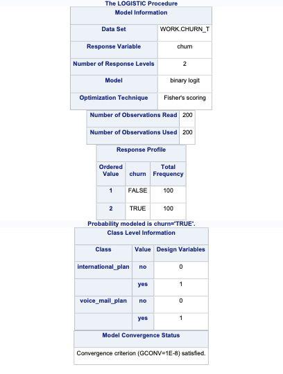
This will produce predicted probabilities for our validation data set than have been adjusted to account for the sampling we did to balance out the data set.
The other technique for adjusting the model for over or under sampling is by building the model with weighted observations so the adjustment happens while building instead of after the fact. In weighting the observations we use weighted MLE instead of plain MLE since each observation doesn’t have the same weight in the estimation of the parameters for our model. The only question now is what are the weights. We derive the weights from the same formula we had for the intercept adjustment. The weight for the rare event is 1, while the weight for the non-event is \(\rho_1\pi_0/\rho_0\pi_1\). For our data set this makes the weights 1 and 18.51 respectively.
Let’s see this approach in each of our softwares!
This is easily done in R by creating a new weight variable in our training data with the ifelse function. If our churn variable takes a value of TRUE then that observation has a weight of 1, while the other observations have a weight of 18.51. From there we build the logistic regression model as we learned in the previous section using the glm function. The only new option is the weights = option where you specify the vector of weights for the training data set so weighted MLE can be performed.
train_u$weight <- ifelse(train_u$churn == 'TRUE', 1, 18.51)

logit.model.w <- glm(churn ~ factor(international_plan) +
                             factor(voice_mail_plan) +
                             total_day_charge +
                             customer_service_calls,
                     data = train_u, family = binomial(link = "logit"),
                     weights = weight)
summary(logit.model.w)
Call:
glm(formula = churn ~ factor(international_plan) + factor(voice_mail_plan) +
    total_day_charge + customer_service_calls, family = binomial(link = "logit"),
    data = train_u, weights = weight)

Coefficients:
                              Estimate Std. Error z value Pr(>|z|)
(Intercept)                   -9.76986    0.69645 -14.028  < 2e-16 ***
factor(international_plan)yes  3.33574    0.32426  10.287  < 2e-16 ***
factor(voice_mail_plan)yes    -1.07459    0.27105  -3.965 7.35e-05 ***
total_day_charge               0.16322    0.01647   9.912  < 2e-16 ***
customer_service_calls         0.72694    0.08809   8.252  < 2e-16 ***
---
Signif. codes:  0 '***' 0.001 '**' 0.01 '*' 0.05 '.' 0.1 ' ' 1

(Dispersion parameter for binomial family taken to be 1)

    Null deviance: 820.53  on 207  degrees of freedom
Residual deviance: 585.50  on 203  degrees of freedom
AIC: 599.9

Number of Fisher Scoring iterations: 6test_u_p_w <- predict(logit.model.w, newdata = test_u, type = "response")
test_u <- data.frame(test_u, 'Pred_w' = test_u_p_w)
head(test_u_p_w) 1 2 3 4 5 6
0.059450043 0.003561721 0.046710480 0.965360041 0.592005413 0.441483322 Now we can analyze our results above knowing that the predictions and model have already been adjusted for our sampling because of the weighted approach. We use the predict function to obtain the predictions from our model and make them a new vector in our validation data set.
This is easily done in Python by creating a new weight variable in our training data with the replace function. If our churn variable takes a value of 1 then that observation has a weight of 1, while the other observations have a weight of 18.51. From there we build the logistic regression model as we learned in the previous section using the GLM.from_formula function. The only new option is the freq_weights = option where you specify the vector of weights for the training data set so weighted MLE can be performed.
from statsmodels.genmod.families import Binomial
from statsmodels.genmod.generalized_linear_model import GLM

train_u['weight'] = train_u.churn.replace({1: 1, 0: 18.51})

log_model_w = GLM.from_formula('churn ~ C(international_plan) + C(voice_mail_plan) + total_day_charge + customer_service_calls', data = train_u, freq_weights = train_u['weight'], family = Binomial()).fit()
log_model_w.summary()| Dep. Variable: | churn | No. Observations: | 208 |
| Model: | GLM | Df Residuals: | 2024.04 |
| Model Family: | Binomial | Df Model: | 4 |
| Link Function: | Logit | Scale: | 1.0000 |
| Method: | IRLS | Log-Likelihood: | -332.21 |
| Date: | Mon, 24 Jun 2024 | Deviance: | 664.41 |
| Time: | 19:32:51 | Pearson chi2: | 2.80e+03 |
| No. Iterations: | 7 | Pseudo R-squ. (CS): | 0.5279 |
| Covariance Type: | nonrobust |
| coef | std err | z | P>|z| | [0.025 | 0.975] | |
| Intercept | -8.2249 | 0.617 | -13.331 | 0.000 | -9.434 | -7.016 |
| C(international_plan)[T.yes] | 2.4463 | 0.300 | 8.155 | 0.000 | 1.858 | 3.034 |
| C(voice_mail_plan)[T.yes] | -0.4999 | 0.296 | -1.688 | 0.091 | -1.080 | 0.081 |
| total_day_charge | 0.1278 | 0.015 | 8.455 | 0.000 | 0.098 | 0.157 |
| customer_service_calls | 0.4614 | 0.076 | 6.091 | 0.000 | 0.313 | 0.610 |
Now we can analyze our results above knowing that the predictions and model have already been adjusted for our sampling because of the weighted approach. We use the predict function to obtain the predictions from our model and make them a new vector in our validation data set.
test_u['pred_w'] = log_model_w.predict(test_u)<string>:1: SettingWithCopyWarning:
A value is trying to be set on a copy of a slice from a DataFrame.
Try using .loc[row_indexer,col_indexer] = value instead
See the caveats in the documentation: https://pandas.pydata.org/pandas-docs/stable/user_guide/indexing.html#returning-a-view-versus-a-copytest_u.head() account_length international_plan ... pred pred_w
0 128 no ... 0.042905 0.075672
1 107 no ... 0.008788 0.008558
2 137 no ... 0.031863 0.050412
3 84 yes ... 0.737190 0.838906
4 75 yes ... 0.389486 0.316033
[5 rows x 11 columns]We use the DATA STEP to create a weights variable in our training data set with these weights. Next, we build the logistic regression model for our training data as we previously learned in the last section, but with the new WEIGHT statement. In this WEIGHT statement we specify the weights variable for PROC LOGISTIC to use these weights for the weighted MLE.
data churn_t;
   set churn_t;
   weights = 1;
   if churn = 'FALSE' then weights = 18.51;
run;proc logistic data=churn_t;
class international_plan(ref='no') voice_mail_plan(ref='no') / param=ref;
model churn(event='TRUE') = international_plan
voice_mail_plan
total_day_charge
customer_service_calls / clodds=pl;
weight weights;
score data=churn_v out=churn_scored2;
run;
quit;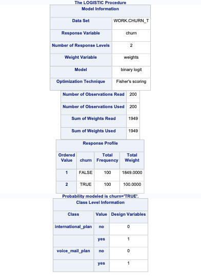
Now we can analyze our results above knowing that the predictions and model have already been adjusted for our sampling because of the weighted approach.
Which approach is better? The more common approach is the weighted observation approach. Empirical simulation studies have shown that for large sample sizes (n > 1000), the weighted approach is better. In small sample sizes (n < 1000), the adjusted intercept approach is only better when you correctly specify the model. In other words, if you plan on doing variable selection because you are unsure if you have the correct variables in your model, then your model may be misspecified in its current form until after your perform variable selection. That being the case, it is probably safer to use the weighted approach. This is why most people use the weighted approach.
Categorical variables can provide great value to any model. Specifically, we might be interested in the differences that might exist across categories in a logistic regression model with regards to our target variable. However, by default, logistic regression models only provide certain categorical comparisons based on the coding of our categorical variables. Through contrasts we can compare any two categories or combination of categories that we desire.
Let’s see how to do this in each of our softwares!
R and the glht function can easily test all combinations of categorical variable categories for inference on the target variable. First we need the variables in a workable format. We need to make the categorical variables factors outside the glm function. This new factor representation of customer_service_calls is represented by the fcsc variable using the factor function. Then we fit our model as usual with the glm function. With the glht function, we test each combination of the levels of the variable for statistical differences. The linfct option specifies the linear function we are trying to test. This option can be used to test all combinations as we do below or individual combinations (like the TEST statement in SAS, but are not shown here). With the mcp function we specify that we want multiple comparisons with the Tukey adjustment on the fcsc variable.
train_u$fcsc <- factor(train_u$customer_service_calls)

logit.model.w.2 <- glm(churn ~ factor(international_plan) +
                               factor(voice_mail_plan) +
                               total_day_charge +
                               fcsc,
                       data = train_u, family = binomial(link = "logit"),
                       weights = weight)
summary(logit.model.w.2)
Call:
glm(formula = churn ~ factor(international_plan) + factor(voice_mail_plan) +
    total_day_charge + fcsc, family = binomial(link = "logit"),
    data = train_u, weights = weight)

Coefficients:
                                Estimate Std. Error z value Pr(>|z|)
(Intercept)                    -10.14898    0.81614 -12.435  < 2e-16 ***
factor(international_plan)yes    3.29320    0.34765   9.473  < 2e-16 ***
factor(voice_mail_plan)yes      -0.99871    0.30330  -3.293 0.000992 ***
total_day_charge                 0.17916    0.01788  10.020  < 2e-16 ***
fcsc1                            0.49930    0.36184   1.380 0.167621
fcsc2                            1.44557    0.40012   3.613 0.000303 ***
fcsc3                            1.22910    0.44653   2.753 0.005913 **
fcsc4                            3.61477    0.51999   6.952 3.61e-12 ***
fcsc5                            2.38244    0.69874   3.410 0.000651 ***
fcsc6                           22.86252  799.55896   0.029 0.977188
fcsc7                           21.52806 1028.81098   0.021 0.983305
---
Signif. codes:  0 '***' 0.001 '**' 0.01 '*' 0.05 '.' 0.1 ' ' 1

(Dispersion parameter for binomial family taken to be 1)

    Null deviance: 820.53  on 207  degrees of freedom
Residual deviance: 545.74  on 197  degrees of freedom
AIC: 571.92

Number of Fisher Scoring iterations: 14library(multcomp)
summary(glht(logit.model.w.2, linfct = mcp(fcsc = "Tukey")))
     Simultaneous Tests for General Linear Hypotheses

Multiple Comparisons of Means: Tukey Contrasts


Fit: glm(formula = churn ~ factor(international_plan) + factor(voice_mail_plan) +
    total_day_charge + fcsc, family = binomial(link = "logit"),
    data = train_u, weights = weight)

Linear Hypotheses:
            Estimate Std. Error z value Pr(>|z|)
1 - 0 == 0    0.4993     0.3618   1.380  0.81745
2 - 0 == 0    1.4456     0.4001   3.613  0.00461 **
3 - 0 == 0    1.2291     0.4465   2.753  0.07439 .
4 - 0 == 0    3.6148     0.5200   6.952  < 0.001 ***
5 - 0 == 0    2.3824     0.6987   3.410  0.00958 **
6 - 0 == 0   22.8625   799.5590   0.029  1.00000
7 - 0 == 0   21.5281  1028.8110   0.021  1.00000
2 - 1 == 0    0.9463     0.3627   2.609  0.10896
3 - 1 == 0    0.7298     0.4043   1.805  0.53232
4 - 1 == 0    3.1155     0.4811   6.476  < 0.001 ***
5 - 1 == 0    1.8831     0.6683   2.818  0.06231 .
6 - 1 == 0   22.3632   799.5589   0.028  1.00000
7 - 1 == 0   21.0288  1028.8109   0.020  1.00000
3 - 2 == 0   -0.2165     0.4001  -0.541  0.99906
4 - 2 == 0    2.1692     0.4649   4.666  < 0.001 ***
5 - 2 == 0    0.9369     0.7019   1.335  0.84161
6 - 2 == 0   21.4170   799.5589   0.027  1.00000
7 - 2 == 0   20.0825  1028.8109   0.020  1.00000
4 - 3 == 0    2.3857     0.4942   4.828  < 0.001 ***
5 - 3 == 0    1.1533     0.7266   1.587  0.68743
6 - 3 == 0   21.6334   799.5589   0.027  1.00000
7 - 3 == 0   20.2990  1028.8109   0.020  1.00000
5 - 4 == 0   -1.2323     0.7743  -1.592  0.68452
6 - 4 == 0   19.2478   799.5589   0.024  1.00000
7 - 4 == 0   17.9133  1028.8110   0.017  1.00000
6 - 5 == 0   20.4801   799.5591   0.026  1.00000
7 - 5 == 0   19.1456  1028.8111   0.019  1.00000
7 - 6 == 0   -1.3345  1302.9759  -0.001  1.00000
---
Signif. codes:  0 '***' 0.001 '**' 0.01 '*' 0.05 '.' 0.1 ' ' 1
(Adjusted p values reported -- single-step method)
In the table above you we have the statistical tests of 28 combinations of the customer_service_calls variable levels. These tests tell us if there is a statistical difference between the two categories with respect to customers churning. You will notice some rather interesting odds ratios and confidence intervals for a couple of the tests. We will talk further about these issues in the convergence section below.
At the time of writing this code deck, Python did not have a built in way to test each of the combinations of categories in a categorical predictor variable against the target variable. That would imply that you would need to loop through many different logistic regressions and change the reference level for the categorical variable in each step of the loop.
SAS and PROC LOGISTIC can easily test all or any combination of categorical variable categories for inference on the target variable. The ODDSRATIO statement allows us to test all possible combinations of a specific categorical variable’s levels. Here we are looking at the customer_service_calls variable which is being treated as a categorical variable. With the diff = all option, we test each combination of the levels of the variable for statistical differences.
ods html select OddsRatiosWald;
proc logistic data=churn_t;
   class international_plan(ref='no') voice_mail_plan(ref='no')
         customer_service_calls(ref='0') / param=ref;
   model churn(event='TRUE') = international_plan
                               voice_mail_plan
                               total_day_charge
                               customer_service_calls / clodds=pl;
   weight weights;
   oddsratio customer_service_calls / diff=all;
run;
quit;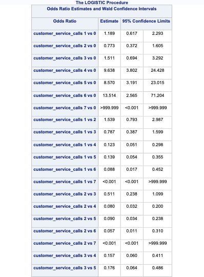
In the table above we have the statistical tests of all 28 combinations of the customer_service_calls variable levels. These tell us if there is a statistical difference between the two categories with respect to customers churning. You will notice some rather interesting odds ratios and confidence intervals for a couple of the tests. We will talk further about these issues in the convergence section below.
If instead you wanted to test certain combinations of the levels as compared to every combination, you can use the TEST statement in PROC LOGISTIC. In the first TEST statement below we are testing if 1 customer service call is equal to two customer service calls in terms of likelihood of churning. The second TEST statement is testing if 1 customer service call is different than the average of 4, 5, 6, and 7 customer service calls (in terms of their categories) with regards to churn. Note the names on these variables. That is the most difficult part of SAS TEST statements. It would probably be best to first run the model to get the names that SAS uses for these variables in the Parameter Estimate output before running their specific tests.
ods html select TestStmts;
proc logistic data=churn_t;
   class international_plan(ref='no') voice_mail_plan(ref='no')
         customer_service_calls(ref='0') / param=ref;
   model churn(event='TRUE') = international_plan
                               voice_mail_plan
                               total_day_charge
                               customer_service_calls / clodds=pl;
   weight weights;
   test customer_service_cal1 = customer_service_cal2;
   test customer_service_cal1 = 0.25*customer_service_cal4 +
                                  0.25*customer_service_cal5 +
                                  0.25*customer_service_cal6 +
                                  0.25*customer_service_cal7;
run;
quit;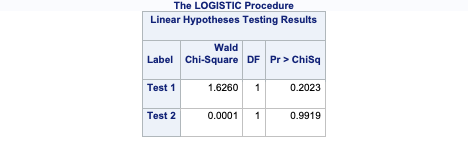
As you can see from the results above, there are no statistical differences in the category combinations we were testing with the TEST statements.
One of the downsides of maximum likelihood estimation is that there is no closed form solution in logistic regression. This means that an algorithm must converge and find the point that maximizes our logistic regression likelihood instead of just calculating a known answer like OLS in linear regression. This means that the algorithm might not converge.
Categorical variables are the typical culprit for causing problems in convergence (however, rarely continuous variables can do this as well). This lack of convergence from categorical variables is from linear separation or quasi-complete separation. Complete linear separation occurs when some combination of the predictors perfectly predict every outcome as you can see in the table below:
| Variable | Yes | No | Logit |
|---|---|---|---|
| Group A | 100 | 0 | Infinity |
| Group B | 0 | 50 | Negative Infinity |
Quasi-complete separation occurs when the outcome can be perfectly predicted for only a subset of the data as shown in the table below:
| Variable | Yes | No | Logit |
|---|---|---|---|
| Group A | 77 | 23 | 1.39 |
| Group B | 0 | 50 | Negative Infinity |
The reason this poses a problem is that the likelihood function doesn’t actually have a maximum.

Remember that the logistic function is completely bounded within 0 and 1. Since these categories perfectly predict the target variable, we need a prediction of 0 or 1 for the probability which cannot be obtained in the logistic regression without infinitely positive (or negative) parameter estimates.
Let’s see if this is a problem in our data set (hint… it is!) and how to address this problem in our software!
Ideally, we should explore all of our categorical variables before we ever model so separation issues shouldn’t be a surprise. Let’s examine our customer_service_calls variable using the table function.
table(train_u$customer_service_calls, train_u$churn)
    FALSE TRUE
  0    29   25
  1    34   25
  2    23   20
  3    15   12
  4     2   13
  5     1    4
  6     0    3
  7     0    2
We can see that the category of 6 customer service calls predicts churn perfectly - 3 person churned while 0 did not. Same for 7 customer service calls. Every other category has at least one person who churned and one who didn’t churn, so this is an example of quasi-complete separation.
In case you don’t explore your data ahead of time, you will notice interesting results in categories with separation issues. Let’s examine the parameter estimates for 6 and 7 customer service calls.
logit.model.w <- glm(churn ~ factor(international_plan) +
                               factor(voice_mail_plan) +
                               total_day_charge +
                               factor(customer_service_calls),
                     data = train_u, family = binomial(link = "logit"),
                     weights = weight)
summary(logit.model.w)
Call:
glm(formula = churn ~ factor(international_plan) + factor(voice_mail_plan) +
    total_day_charge + factor(customer_service_calls), family = binomial(link = "logit"),
    data = train_u, weights = weight)

Coefficients:
                                  Estimate Std. Error z value Pr(>|z|)
(Intercept)                      -10.14898    0.81614 -12.435  < 2e-16 ***
factor(international_plan)yes      3.29320    0.34765   9.473  < 2e-16 ***
factor(voice_mail_plan)yes        -0.99871    0.30330  -3.293 0.000992 ***
total_day_charge                   0.17916    0.01788  10.020  < 2e-16 ***
factor(customer_service_calls)1    0.49930    0.36184   1.380 0.167621
factor(customer_service_calls)2    1.44557    0.40012   3.613 0.000303 ***
factor(customer_service_calls)3    1.22910    0.44653   2.753 0.005913 **
factor(customer_service_calls)4    3.61477    0.51999   6.952 3.61e-12 ***
factor(customer_service_calls)5    2.38244    0.69874   3.410 0.000651 ***
factor(customer_service_calls)6   22.86252  799.55896   0.029 0.977188
factor(customer_service_calls)7   21.52806 1028.81098   0.021 0.983305
---
Signif. codes:  0 '***' 0.001 '**' 0.01 '*' 0.05 '.' 0.1 ' ' 1

(Dispersion parameter for binomial family taken to be 1)

    Null deviance: 820.53  on 207  degrees of freedom
Residual deviance: 545.74  on 197  degrees of freedom
AIC: 571.92

Number of Fisher Scoring iterations: 14
Notice the category of 6 and 7 compared to the rest. Their parameter estimates are rather high (remember that odds ratios are exponentiated parameter estimates so 20+ is REALLY large). These are definite signs of convergence problems, especially considering the p-value for these is close to 1!
Once possible solution to convergence problems in logistic regression is to perform exact logistic regression. This method is computationally more expensive and should really only be used if you need an estimate for the specific category that is causing the separation issues. The logistf package in R can perform this analysis but is not shown here.
A more common solution to separation concerns is to transform the categorical variable. Instead of having a category with separation issues, you can combine this category with another category to remove the separation concerns. Below we are creating a “4+” category that contains the categories of 4, 5, 6, and 7. This will remove the separation issues as you can see as we rerun the logistic regression.
train_u$customer_service_calls_c <- as.character(train_u$customer_service_calls)
train_u$customer_service_calls_c[which(train_u$customer_service_calls > 3)] <- "4+"

table(train_u$customer_service_calls_c, train_u$churn)
     FALSE TRUE
  0     29   25
  1     34   25
  2     23   20
  3     15   12
4+ 3 22logit.model.w <- glm(churn ~ factor(international_plan) +
factor(voice_mail_plan) +
total_day_charge +
factor(customer_service_calls_c),
data = train_u, family = binomial(link = "logit"),
weights = weight)
summary(logit.model.w)
Call:
glm(formula = churn ~ factor(international_plan) + factor(voice_mail_plan) +
    total_day_charge + factor(customer_service_calls_c), family = binomial(link = "logit"),
    data = train_u, weights = weight)

Coefficients:
                                   Estimate Std. Error z value Pr(>|z|)
(Intercept)                        -9.18049    0.73431 -12.502  < 2e-16 ***
factor(international_plan)yes       3.08132    0.33255   9.266  < 2e-16 ***
factor(voice_mail_plan)yes         -1.14286    0.27819  -4.108 3.99e-05 ***
total_day_charge                    0.15726    0.01647   9.551  < 2e-16 ***
factor(customer_service_calls_c)1   0.44991    0.35419   1.270  0.20400
factor(customer_service_calls_c)2   1.25333    0.38493   3.256  0.00113 **
factor(customer_service_calls_c)3   1.03757    0.43343   2.394  0.01667 *
factor(customer_service_calls_c)4+  3.45947    0.42510   8.138 4.02e-16 ***
---
Signif. codes:  0 '***' 0.001 '**' 0.01 '*' 0.05 '.' 0.1 ' ' 1

(Dispersion parameter for binomial family taken to be 1)

    Null deviance: 820.53  on 207  degrees of freedom
Residual deviance: 580.00  on 200  degrees of freedom
AIC: 600.53

Number of Fisher Scoring iterations: 6
Notice how we no longer have the large parameter estimates since we have corrected our converge problems.
Ideally, we should explore all of our categorical variables before we ever model so separation issues shouldn’t be a surprise. Let’s examine our customer_service_calls variable using the crosstab function.
pd.crosstab(index = train_u['churn'], columns = train_u['customer_service_calls'])customer_service_calls 0 1 2 3 4 5 6 7
churn
0 27 38 23 13 1 1 1 0
1 21 26 20 10 16 7 3 1We can see that the category of 7 customer service calls predicts churn perfectly - 1 person churned while 0 did not. Every other category has at least one person who churned and one who didn’t so this is an example of quasi-complete separation.
In case you don’t explore your data ahead of time, you will notice interesting results in categories with separation issues. Let’s examine the parameter estimates for 7 customer service calls.
log_model_w = GLM.from_formula('churn ~ C(international_plan) + C(voice_mail_plan) + total_day_charge + C(customer_service_calls)', data = train_u, freq_weights = train_u['weight'], family = Binomial()).fit()
log_model_w.summary()| Dep. Variable: | churn | No. Observations: | 208 |
| Model: | GLM | Df Residuals: | 2018.04 |
| Model Family: | Binomial | Df Model: | 10 |
| Link Function: | Logit | Scale: | 1.0000 |
| Method: | IRLS | Log-Likelihood: | -317.52 |
| Date: | Mon, 24 Jun 2024 | Deviance: | 635.04 |
| Time: | 19:32:53 | Pearson chi2: | 2.73e+03 |
| No. Iterations: | 19 | Pseudo R-squ. (CS): | 0.5901 |
| Covariance Type: | nonrobust |
| coef | std err | z | P>|z| | [0.025 | 0.975] | |
| Intercept | -8.0706 | 0.657 | -12.285 | 0.000 | -9.358 | -6.783 |
| C(international_plan)[T.yes] | 2.0280 | 0.353 | 5.746 | 0.000 | 1.336 | 2.720 |
| C(voice_mail_plan)[T.yes] | -0.5006 | 0.298 | -1.677 | 0.093 | -1.085 | 0.084 |
| C(customer_service_calls)[T.1] | -0.0310 | 0.321 | -0.097 | 0.923 | -0.659 | 0.597 |
| C(customer_service_calls)[T.2] | -0.1296 | 0.346 | -0.375 | 0.708 | -0.807 | 0.548 |
| C(customer_service_calls)[T.3] | -0.0181 | 0.420 | -0.043 | 0.966 | -0.841 | 0.805 |
| C(customer_service_calls)[T.4] | 2.3836 | 0.485 | 4.919 | 0.000 | 1.434 | 3.333 |
| C(customer_service_calls)[T.5] | 2.7124 | 0.534 | 5.078 | 0.000 | 1.666 | 3.759 |
| C(customer_service_calls)[T.6] | 2.1312 | 0.688 | 3.096 | 0.002 | 0.782 | 3.480 |
| C(customer_service_calls)[T.7] | 25.2870 | 1.77e+04 | 0.001 | 0.999 | -3.47e+04 | 3.48e+04 |
| total_day_charge | 0.1415 | 0.016 | 8.573 | 0.000 | 0.109 | 0.174 |
Notice the category of 7 compared to the rest. It’s parameter estimates is rather high (remember that odds ratios are exponentiated parameter estimates so 20+ is REALLY large). That is a definite sign of convergence problems, especially since the p-value is close to 1!
Once possible solution to convergence problems in logistic regression is to perform exact logistic regression. This method is computationally more expensive and should really only be used if you need an estimate for the specific category that is causing the separation issues. At the time of writing this code deck, there was no way to perform this in Python.
A more common solution to separation concerns is to transform the categorical variable. Instead of having a category with separation issues, you can combine this category with another category to remove the separation concerns. Below we are creating a “4+” category that contains the categories of 4, 5, 6, and 7. This will remove the separation issues as you can see as we rerun the logistic regression.
train_u['customer_service_calls_c'] = train_u['customer_service_calls']

train_u.loc[train_u['customer_service_calls'] >= 4, ['customer_service_calls_c']] = 4

pd.crosstab(index = train_u['churn'], columns = train_u['customer_service_calls_c'])
customer_service_calls_c 0 1 2 3 4
churn
0 27 38 23 13 3
1 21 26 20 10 27log_model_w = GLM.from_formula('churn ~ C(international_plan) + C(voice_mail_plan) + total_day_charge + C(customer_service_calls_c)', data = train_u, freq_weights = train_u['weight'], family = Binomial()).fit()
log_model_w.summary()| Dep. Variable: | churn | No. Observations: | 208 |
| Model: | GLM | Df Residuals: | 2021.04 |
| Model Family: | Binomial | Df Model: | 7 |
| Link Function: | Logit | Scale: | 1.0000 |
| Method: | IRLS | Log-Likelihood: | -320.16 |
| Date: | Mon, 24 Jun 2024 | Deviance: | 640.32 |
| Time: | 19:32:53 | Pearson chi2: | 2.64e+03 |
| No. Iterations: | 7 | Pseudo R-squ. (CS): | 0.5795 |
| Covariance Type: | nonrobust |
| coef | std err | z | P>|z| | [0.025 | 0.975] | |
| Intercept | -7.9854 | 0.638 | -12.508 | 0.000 | -9.237 | -6.734 |
| C(international_plan)[T.yes] | 1.9624 | 0.315 | 6.224 | 0.000 | 1.344 | 2.580 |
| C(voice_mail_plan)[T.yes] | -0.5085 | 0.297 | -1.710 | 0.087 | -1.091 | 0.074 |
| C(customer_service_calls_c)[T.1] | -0.0381 | 0.319 | -0.119 | 0.905 | -0.663 | 0.587 |
| C(customer_service_calls_c)[T.2] | -0.1339 | 0.344 | -0.389 | 0.697 | -0.809 | 0.541 |
| C(customer_service_calls_c)[T.3] | -0.0313 | 0.417 | -0.075 | 0.940 | -0.849 | 0.787 |
| C(customer_service_calls_c)[T.4] | 2.4978 | 0.363 | 6.888 | 0.000 | 1.787 | 3.209 |
| total_day_charge | 0.1396 | 0.016 | 8.602 | 0.000 | 0.108 | 0.171 |
Notice how we no longer have the large parameter estimates since we have corrected our convergence problems.
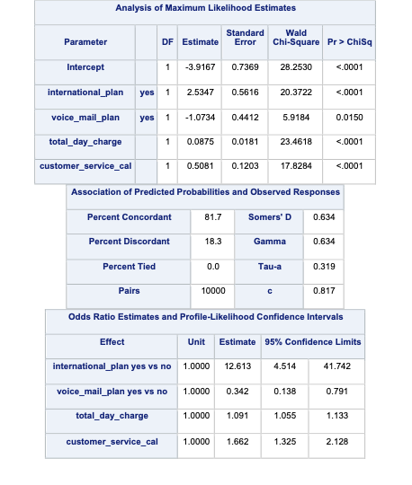
Ideally, we should explore all of our categorical variables before we ever model so separation issues shouldn’t be a surprise. Let’s examine our customer_service_calls variable using PROC FREQ.
proc freq data=churn_t;
   table customer_service_calls*churn;
run;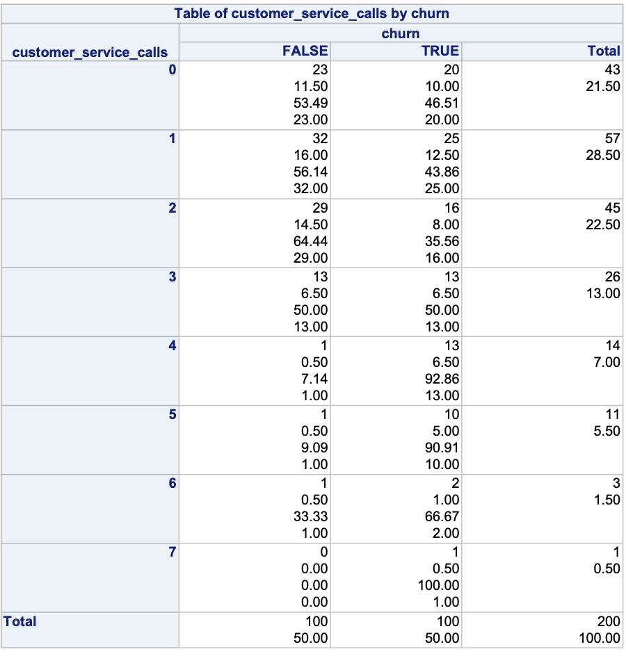
We can see that the category of 7 customer service calls predicts churn perfectly - 1 person churned while 0 did not. Every other category has at least one person who churned and one who didn’t so this is an example of quasi-complete separation.
In case you don’t explore your data ahead of time, you will notice interesting results in categories with separation issues. Let’s examine the parameter estimates for 6 and 7 customer service calls.
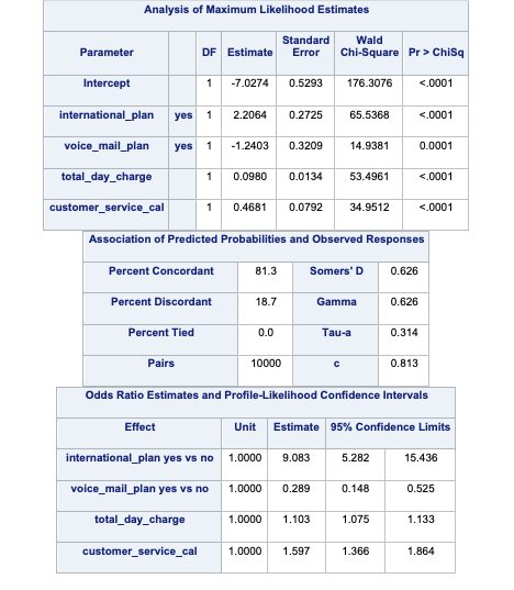
ods html select ParameterEstimates;
proc logistic data=churn_t;
   class international_plan(ref='no') voice_mail_plan(ref='no')
         customer_service_calls(ref='0') / param=ref;
   model churn(event='TRUE') = international_plan
                               voice_mail_plan
                               total_day_charge
                               customer_service_calls / clodds=pl;
   weight weights;
run;
quit;.png)
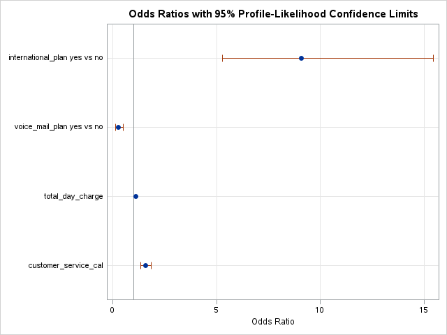
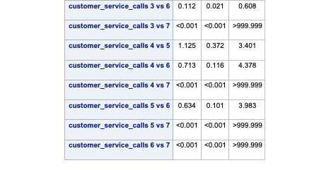
Notice the category of 7 compared to that of 6. Its parameter estimate is rather high (remember that odds ratios are exponentiated parameter estimates close to 20 are REALLY large). Also notice the inflated standard error in the thousands as compared to single digits for the 7 category. This leads to a test statistic basically equal to 0 with a really high p-value. These are definite signs of convergence problems!
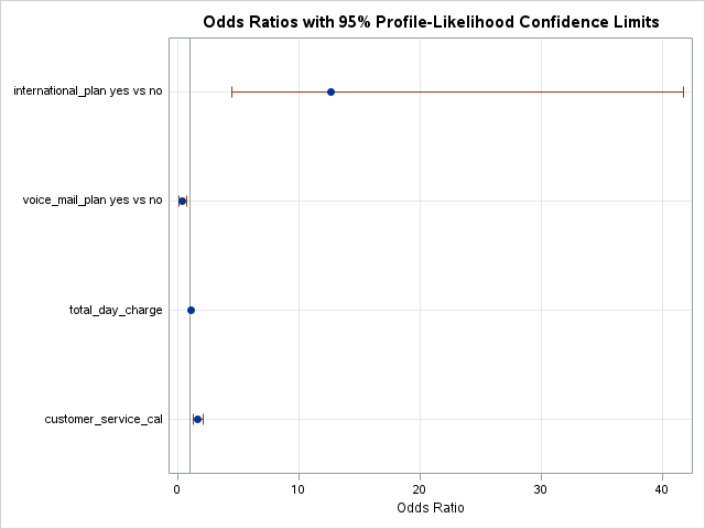
Once possible solution to convergence problems in logistic regression is to perform exact logistic regression. This method is computationally more expensive and should really only be used if you need an estimate for the specific category that is causing the separation issues. The firth option in PROC LOGISTIC can perform this analysis. The code is shown below with limited output.
ods html select ParameterEstimates;
proc logistic data=churn_t;
   class international_plan(ref='no') voice_mail_plan(ref='no')
         customer_service_calls(ref='0') / param=ref;
   model churn(event='TRUE') = international_plan
                               voice_mail_plan
                               total_day_charge
                               customer_service_calls / firth;
   weight weights;
run;
quit;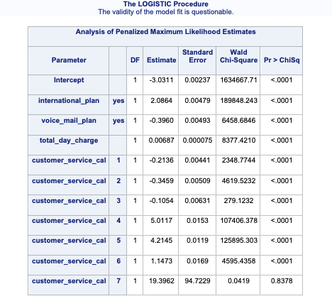
A more common solution to separation concerns is to transform the categorical variable. Instead of having a category with separation issues, you can combine this category with another category to remove the separation concerns. Below we are creating a “4+” category that contains the categories of 4, 5, 6, and 7. This will remove the separation issues as you can see as we rerun the logistic regression.
data churn_t;
   set churn_t;
   customer_service_calls_c = put(customer_service_calls, 2.);;
   if customer_service_calls > 3 then customer_service_calls_c = '4+';
run;

ods html select ParameterEstimates;
proc logistic data=churn_t;
   class international_plan(ref='no') voice_mail_plan(ref='no')
         customer_service_calls_c(ref='0') / param=ref;
   model churn(event='TRUE') = international_plan
                               voice_mail_plan
                               total_day_charge
                               customer_service_calls_c / clodds=pl;
   weight weights;
run;
quit;
Notice how we no longer have the large parameter estimates since we have corrected our convergence problems.
Ordinal variables are easy to combine categories because you can just combine separation categories with categories on either side. However, with nominal variables we typically combine the separation causing category with the category that has the relationship with the target variable that is the most similar. The following plot is an example of this:
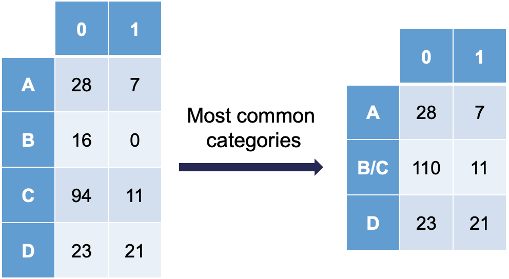
Notice how category C is most similar to category B (the problem category) in terms of its ratio of 0’s and 1’s. Formally, this method of combining categories is also called the Greenacre method.