Recent Developments

Change

The field of risk management is ever changing and growing quickly. The following couple of sections outline some of the latest additions to the field of risk management - extreme value theory (EVT) and newer VaR calculations.

Extreme Value Theory

There are some complications to the expected shortfall calculation. First, ES estimates tend to be less stable than the VaR for the same confidence level due to sample size limitations. ES requires a large number of observations to generate a reliable estimate. Due to this, ES is also more sensitive to estimation errors than VaR because is substantially depends on the accuracy of the tail model used in the distribution.

We try so hard to estimate the full distribution. However, our only care is the tail of the distribution so we will turn our attention on just estimating the tail. This is the value of extreme value theory (EVT). EVT provides the theoretical foundation for building statistical models describing extreme events. This is used in many fields such as finance, structual engineering, traffic prediction, weather prediction, and geological prediction.

EVT provides the distribution for the following two things:

Block Maxima (Minima) - the maximum (or minimum) the variable takes in successive periods.
Exceedances - the values that exceed a certain threshold.

For VaR and ES calculations we will focus on the exceedances piece of EVT. The approach of exceedances tries to understand the distribution of values that exceed a certain threshold. Instead of isolating the tail of an overall distribution (limiting the values) we are trying to build a distribution for the tail events themselves.

One of the popular distributions for this is the generalized Pareto. This distribution is named after Italian engineer and economist Vilfredo Pareto. It came into popularity with the “Pareto Principle” which is more commonly known as the “80-20” Rule. Pareto noted in 1896 that 80% of the land of Italy was owned by 20% of the population. Richard Koch authored the book The 80/20 Principle to illustrate some common applications. The plot below shows some example Pareto distributions:

This can be applied to value at risk and expected shortfall to provide more accurate estimates of VaR and ES, but the math is very complicated. We need to use maximum likelihood estimation to find which generalized Pareto distribution fits our data the best - which parameters $\xi$ and $\beta$ are optimal to maximize:

\[ f(v) = \sum_{i=1}^{n_u} \log(\frac{1}{\beta} \times (1 + \frac{\xi (v_i - u)}{\beta})^{\frac{-1}{\xi -1}}) \]

The calculation for VaR from the Pareto distribution is:

\[ VaR = u + \frac{\beta}{\xi}([\frac{n}{n_u}(1-q)]^{-\xi}) \]

The calculation of ES from the Pareto distribution is:

\[ ES = \frac{VaR + \beta - \xi u}{1- \xi} \]

Let’s walk through the approach for our two position portfolio. If we have $200,000 invested in Microsoft and $100,000 invested in Apple, we can use the 500 observations for each stocks’ returns to estimate the generalized Pareto distribution parameters. Assume a normal distribution for each of these stocks returns with their historical mean and standard deviation. From there we can just estimate the VaR and ES from the above equations.

Let’s see how to this in each of our softwares!

To get the estimated parameters from the Pareto distribution we can use the gpdFit function. The first input is the data itself (careful, the function requires positive values) and the second input input is the type = c("mle") option to specify using maximum likelihood estimation to estimate the parameters. From there we use the tailRisk function to estimate the VaR and ES from the output of the gpdFit function.

Code

library(fExtremes)
library(scales)

pareto.fit <-gpdFit(as.numeric(stocks$port_v[-1])*-1, type = c("mle"))
tailRisk(pareto.fit, prob = 0.99)

    Prob      VaR       ES
95% 0.99 13884.16 15710.78

Code

dollar(tailRisk(pareto.fit, prob = 0.99)[,2]*-1)

[1] "-$13,884.16"

Code

dollar(tailRisk(pareto.fit, prob = 0.99)[,3]*-1)

[1] "-$15,710.78"

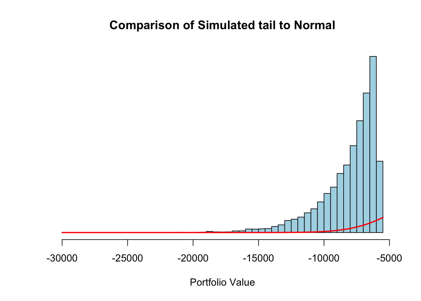
We can see the values from the Pareto estimation above. To compare this to the normal distribution, the following plot shows the estimated distribution (in the histogram) of the Pareto distribution compared to the theoretical normal distribution (the density line) for the same data.

Code

hist(-1*rgpd(n = 10000, mu = pareto.fit@parameter$u, beta = pareto.fit@fit$par.ests[2], xi = pareto.fit@fit$par.ests[1]), breaks = 50, main = "Comparison of Simulated tail to Normal", xlab = "Portfolio Value", freq = FALSE, yaxt = "n", ylab = "", col = "lightblue")
curve(dnorm(x, mean(stocks$port_v, na.rm = TRUE), sd(stocks$port_v, na.rm = TRUE)), add = TRUE, col = 'red', lwd = 2)

To get the estimated parameters from the Pareto distribution we can use the pareto.fit function from scipy.stats. The first input is the data itself (careful, the function requires positive values). We use a smaller sample of our data since the tail of the data is what we believe follows the Pareto. From there we use the random.pareto function to simulate many values from a Pareto distribution with parameters estimated from the pareto.fit function. Then we use the quantile function estimate the VaR and ES from the output of the random.pareto function.

Code

import scipy.stats as sps
import numpy as np
import locale

VaR_percentile = 0.01
AAPL_inv = 100000
MSFT_inv = 200000

par_stocks = stocks['port_v'].sort_values().head(48)*(-1)

shape, loc, scale = sps.pareto.fit(par_stocks)

ran_pareto = np.random.pareto(shape, size = 1000)*scale - loc

VaR_EVT = np.quantile(ran_pareto, (1-VaR_percentile))
locale.currency(VaR_EVT, grouping = True)

'$22,293.89'

Code

ES_EVT = np.mean(ran_pareto[ran_pareto > np.quantile(ran_pareto, (1-VaR_percentile))])
locale.currency(ES_EVT, grouping = True)

'$26,258.82'

In SAS, we first need to isolate the tail fo the data to fit the Pareto distribution with. SAS requires that the data values are all positive so we convert our negative values to positive using the DATA step and multiplying our values by -1. Next, we use PROC UNIVARIATE to calculate the percentiles of our data. We want to isolate the 5% tail to build our Pareto distribution off of. We specify the variable of interest, neg_port_v, in our VAR statement. We then use the OUTPUT statement to save the percentiles into a new dataset called percentiles by using the pctlpts = 95 and pctlpre = P options we have defined before. Next, we use another DATA step to create a MACRO variable for the value of the 5% quantile of interest (remember we are working with the 95% instead of 5% because we flipped all of our values when taking the negative). We then use a last DATA step to delete all the data values not in the tail of interest.

Code

%let var_percentile=0.01;

data neg_stocks;
    set SimRisk.stocks;
    neg_port_v = -1*port_v;
run;

proc univariate data=neg_stocks;
    var neg_port_v;
    output out=percentiles pctlpts = 95 pctlpre=P;
  ods select Quantiles;
run;

proc print data=percentiles;
run;

data _null_;
    set percentiles;
    call symput("tail",P95);
run;

data stocks_tail;
    set neg_stocks;
    if neg_port_v <= &tail then delete;
run;

Now we can use PROC UNIVARIATE to fit our data to the Pareto distribution. To do this we use the HISTOGRAM statement on our variable neg_port_v with the pareto(theta=&tail percent=80) option. This will fit the parameters of the Pareto distribution to our dataset. We can output these parameters using the ODS OUTPUT statements. The output from PROC UNIVARIATE provides the parameter estimates for the Pareto distribution as well as the estimate of our quantile of interest, the VaR. We save this VaR as a MACRO variable and print it out using PROC IML.

Code

proc univariate data=stocks_tail;
    histogram neg_port_v / pareto(theta=&tail percent=80);
    ods output ParameterEstimates=PE FitQuantiles=FQ;
    ods select histogram ParameterEstimates FitQuantiles;
run;

data _null_;
    set PE;
    if upcase(Symbol) eq 'THETA' then do;
        call symput("threshold",Estimate);
    end;
    if upcase(Symbol) eq 'SIGMA' then do;
        call symput("beta",Estimate);
    end;
    if upcase(Symbol) eq 'ALPHA' then do;
        call symput("xi",Estimate);
    end;
run;

data _null_;
    set FQ;
    call symput("VaR",EstQuantile);
run;

proc iml;
title 'EVT Results';

VaR_EVT = &VaR*-1;

print "Daily VaR (Percentile level: &var_percentile); EVT" VaR_EVT[format=dollar15.2];

quit;

Lastly, we use one final PROC IML call to calculate the ES using the equation defined above.

Code

proc iml;
title 'EVT Results';

VaR_EVT = &VaR*-1;
ES_EVT = ((&VaR + &beta - &xi*&threshold)/(1-&xi))*-1;

print "Daily CVaR/ES (Percentile level: &var_percentile); EVT" ES_EVT[format=dollar15.2];

quit;

These values align with the historical simulation approach that had a much riskier value for VaR and ES compared to the Delta-Normal approach.

VaR Extensions

The last section just briefly touches on some of the latest variations and adaptions of the value at risk metric. There are many additions to VaR calculations:

Delta-Gamma VaR
Delta-Gamma Monte Carlo Simulation
Marginal VaR
Incremental VaR
Component VaR

Let’s discuss each briefly in concept.

The Delta-Gamma approximation approach tries to improve on the Delta-Normal approach by taking into account higher derivatives than the first derivative only. In the expansion of the derivatives we can look at the first two:

\[ dV = \frac{\partial V}{\partial RF} \cdot dRF + \frac{1}{2} \cdot \frac{\partial^2 V}{\partial RF^2} + \cdots \]

\[ dV = \Delta \cdot dRF + \frac{1}{2} \cdot \Gamma \cdot dRF^2 \]

Essentially, this approach takes the variance component into account in building the Gamma portion of the equation. Delta-Normal typically underestimates VaR when assumptions do not hold. The Delta-Gamma approach tries to correct for this, but it is computationally more intensive.

The assumption of normality still might not be reliable even with the Delta-Gamma adjustment to Delta-Normal. The Delta-Gamma MC simulation approach simulates the risk factor before using Taylor-series expansion to create simulated movements in the portfolio’s value. Just like with regular simulation, the VaR is calculated using the simulated distribution of the portfolio.

For a comparison, if you have a large number of things to evaluate in a portfolio with few options, the Delta-Normal approach is fast and efficient enough. However, if you have only a few sources of risk and substantial complexity, the Delta-Gamma approach is better. If you have both a large number of risk factors and substantial complexity, simulation is probably the best approach.

The marginal VaR tries to answer the question of how much the VaR will change if we invest one more dollar in a position of the portfolio. In other words, the first derivative of VaR with respect to the weight of a certain position in the portfolio. Assuming normality, this calculation is quite easy:

\[ \Delta VaR = \alpha \times \frac{Cov(R_i, R_p)}{\sigma_p} \]

The incremental VaR tries to measure the change in VaR due to the addition of a new position in the portfolio. This is used whenever an institution wants to evaluate the effect of a proposed trade or change in the portfolio of interest. This is slightly different from the marginal VaR that only takes into account an additional dollar of one position instead of adding or subtracting an entire (or multiple) positions.

This is trickier to calculate as you now need to calculate the VaR under both portfolios and take their difference. There are Taylor series approximations to his, but they are not as accurate as calculating the full VaR for both portfolios and looking at the difference.

The component VaR decomposes the VaR into its basic components ina way that takes into account the diversification of the portfolio. It is a “partition” of the portfolio VaR that indicates the change of VaR if a given component was deleted. The component VaR is defined in terms of the marginal VaR:

\[ VaR_{Comp} = \Delta VaR \times (\$ \text{ value of component}) \]

The sum of all component VaR’s is the total portfolio VaR.

--- title: "Recent Developments" format: html: code-fold: show code-tools: true editor: visual --- # Change The field of risk management is ever changing and growing quickly. The following couple of sections outline some of the latest additions to the field of risk management - extreme value theory (EVT) and newer VaR calculations. # Extreme Value Theory There are some complications to the expected shortfall calculation. First, ES estimates tend to be less stable than the VaR for the same confidence level due to sample size limitations. ES requires a large number of observations to generate a reliable estimate. Due to this, ES is also more sensitive to estimation errors than VaR because is substantially depends on the accuracy of the tail model used in the distribution. We try so hard to estimate the full distribution. However, our only care is the tail of the distribution so we will turn our attention on just estimating the tail. This is the value of **extreme value theory (EVT)**. EVT provides the theoretical foundation for building statistical models describing extreme events. This is used in many fields such as finance, structual engineering, traffic prediction, weather prediction, and geological prediction. EVT provides the distribution for the following two things: - **Block Maxima (Minima)** - the maximum (or minimum) the variable takes in successive periods. - **Exceedances** - the values that exceed a certain threshold. For VaR and ES calculations we will focus on the exceedances piece of EVT. The approach of exceedances tries to understand the distribution of values that exceed a certain threshold. Instead of isolating the tail of an overall distribution (limiting the values) we are trying to build a distribution for the tail events themselves. One of the popular distributions for this is the **generalized Pareto**. This distribution is named after Italian engineer and economist Vilfredo Pareto. It came into popularity with the "Pareto Principle" which is more commonly known as the "80-20" Rule. Pareto noted in 1896 that 80% of the land of Italy was owned by 20% of the population. Richard Koch authored the book *The 80/20 Principle* to illustrate some common applications. The plot below shows some example Pareto distributions: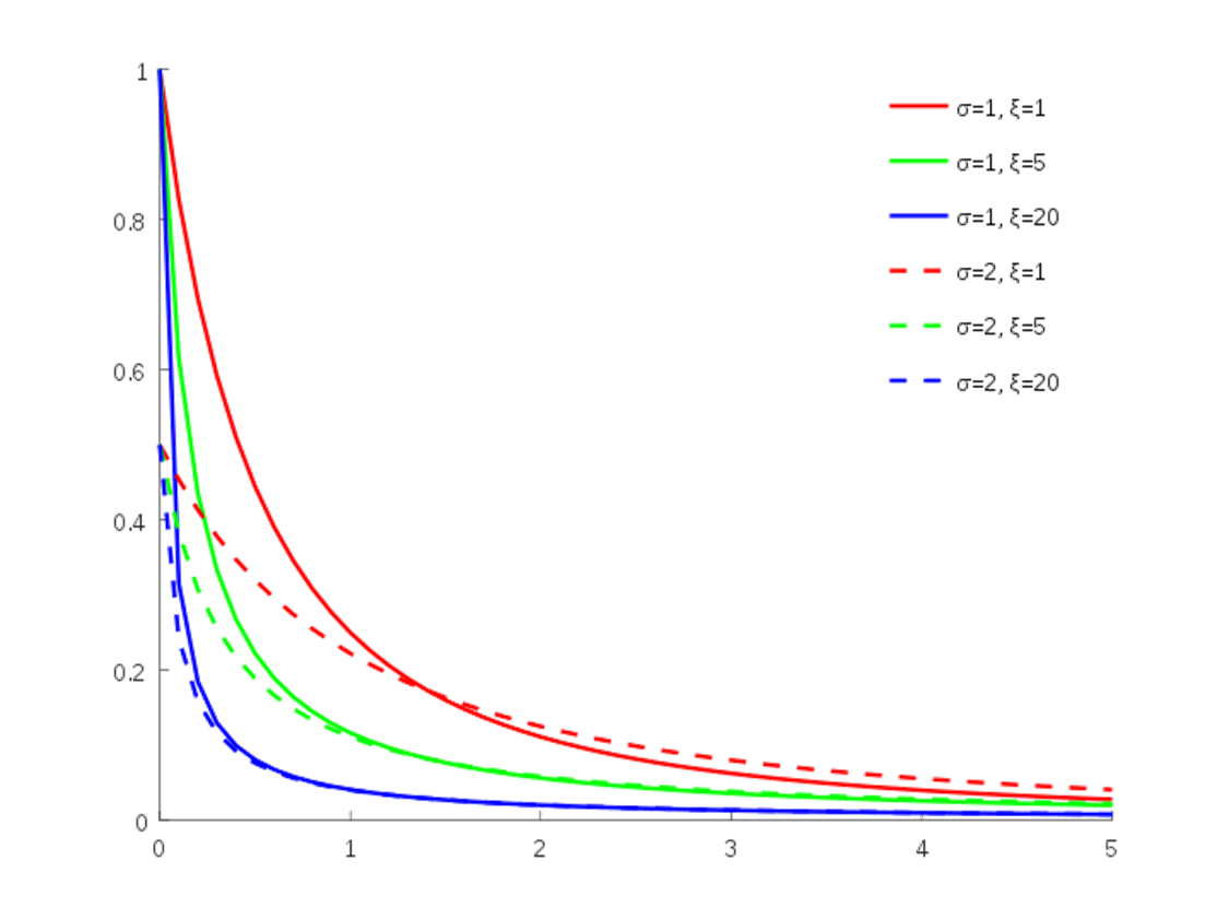 ![Pareto Distribution Example](image/Pareto.png){fig-align="center" width="5in"} This can be applied to value at risk and expected shortfall to provide more accurate estimates of VaR and ES, but the math is very complicated. We need to use maximum likelihood estimation to find which generalized Pareto distribution fits our data the best - which parameters $\xi$ and $\beta$ are optimal to maximize: $$ f(v) = \sum_{i=1}^{n_u} \log(\frac{1}{\beta} \times (1 + \frac{\xi (v_i - u)}{\beta})^{\frac{-1}{\xi -1}}) $$ The calculation for VaR from the Pareto distribution is: $$ VaR = u + \frac{\beta}{\xi}([\frac{n}{n_u}(1-q)]^{-\xi}) $$ The calculation of ES from the Pareto distribution is: $$ ES = \frac{VaR + \beta - \xi u}{1- \xi} $$ Let's walk through the approach for our two position portfolio. If we have \$200,000 invested in Microsoft and \$100,000 invested in Apple, we can use the 500 observations for each stocks' returns to estimate the generalized Pareto distribution parameters. Assume a normal distribution for each of these stocks returns with their historical mean and standard deviation. From there we can just estimate the VaR and ES from the above equations. Let's see how to this in each of our softwares! ::: {.panel-tabset .nav-pills} ## R To get the estimated parameters from the Pareto distribution we can use the `gpdFit` function. The first input is the data itself (careful, the function requires positive values) and the second input input is the `type = c("mle")` option to specify using maximum likelihood estimation to estimate the parameters. From there we use the `tailRisk` function to estimate the VaR and ES from the output of the `gpdFit` function. ```{r} #| echo: false #| message: false #| include: false library(quantmod) tickers = c("AAPL", "MSFT") getSymbols(tickers) stocks <- cbind(last(AAPL[,4], '500 days'), last(MSFT[,4], '500 days')) stocks$msft_r <- ROC(stocks$MSFT.Close) stocks$aapl_r <- ROC(stocks$AAPL.Close) VaR.percentile = 0.01 AAPL.inv <- 100000 MSFT.inv <- 200000 stocks$port_v <- MSFT.inv*stocks$msft_r + AAPL.inv*stocks$aapl_r stocks_df = data.frame(stocks) ``` ```{python} #| echo: false #| message: false #| include: false stocks = r.stocks_df ``` ```{r} library(fExtremes) library(scales) pareto.fit <-gpdFit(as.numeric(stocks$port_v[-1])*-1, type = c("mle")) tailRisk(pareto.fit, prob = 0.99) dollar(tailRisk(pareto.fit, prob = 0.99)[,2]*-1) dollar(tailRisk(pareto.fit, prob = 0.99)[,3]*-1) ``` We can see the values from the Pareto estimation above. To compare this to the normal distribution, the following plot shows the estimated distribution (in the histogram) of the Pareto distribution compared to the theoretical normal distribution (the density line) for the same data. ```{r} hist(-1*rgpd(n = 10000, mu = pareto.fit@parameter$u, beta = pareto.fit@fit$par.ests[2], xi = pareto.fit@fit$par.ests[1]), breaks = 50, main = "Comparison of Simulated tail to Normal", xlab = "Portfolio Value", freq = FALSE, yaxt = "n", ylab = "", col = "lightblue") curve(dnorm(x, mean(stocks$port_v, na.rm = TRUE), sd(stocks$port_v, na.rm = TRUE)), add = TRUE, col = 'red', lwd = 2) ``` ## Python To get the estimated parameters from the Pareto distribution we can use the `pareto.fit` function from `scipy.stats`. The first input is the data itself (careful, the function requires positive values). We use a smaller sample of our data since the tail of the data is what we believe follows the Pareto. From there we use the `random.pareto` function to simulate many values from a Pareto distribution with parameters estimated from the `pareto.fit` function. Then we use the `quantile` function estimate the VaR and ES from the output of the `random.pareto` function. ```{python} import scipy.stats as sps import numpy as np import locale VaR_percentile = 0.01 AAPL_inv = 100000 MSFT_inv = 200000 par_stocks = stocks['port_v'].sort_values().head(48)*(-1) shape, loc, scale = sps.pareto.fit(par_stocks) ran_pareto = np.random.pareto(shape, size = 1000)*scale - loc VaR_EVT = np.quantile(ran_pareto, (1-VaR_percentile)) locale.currency(VaR_EVT, grouping = True) ES_EVT = np.mean(ran_pareto[ran_pareto > np.quantile(ran_pareto, (1-VaR_percentile))]) locale.currency(ES_EVT, grouping = True) ``` ## SAS In SAS, we first need to isolate the tail fo the data to fit the Pareto distribution with. SAS requires that the data values are all positive so we convert our negative values to positive using the `DATA` step and multiplying our values by -1. Next, we use `PROC UNIVARIATE` to calculate the percentiles of our data. We want to isolate the 5% tail to build our Pareto distribution off of. We specify the variable of interest, *neg_port_v*, in our `VAR` statement. We then use the `OUTPUT` statement to save the percentiles into a new dataset called *percentiles* by using the `pctlpts = 95` and `pctlpre = P` options we have defined before. Next, we use another `DATA` step to create a MACRO variable for the value of the 5% quantile of interest (remember we are working with the 95% instead of 5% because we flipped all of our values when taking the negative). We then use a last `DATA` step to delete all the data values not in the tail of interest. ```{r} #| eval: false %let var_percentile=0.01; data neg_stocks; set SimRisk.stocks; neg_port_v = -1*port_v; run; proc univariate data=neg_stocks; var neg_port_v; output out=percentiles pctlpts = 95 pctlpre=P; ods select Quantiles; run; proc print data=percentiles; run; data _null_; set percentiles; call symput("tail",P95); run; data stocks_tail; set neg_stocks; if neg_port_v <= &tail then delete; run;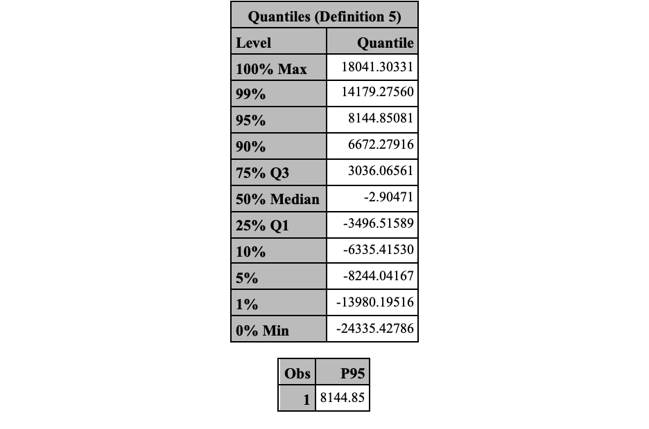 ``` ![](image/3_1a_SAS.png){fig-align="center" width="8in"} Now we can use `PROC UNIVARIATE` to fit our data to the Pareto distribution. To do this we use the `HISTOGRAM` statement on our variable *neg_port_v* with the `pareto(theta=&tail percent=80)` option. This will fit the parameters of the Pareto distribution to our dataset. We can output these parameters using the `ODS OUTPUT` statements. The output from `PROC UNIVARIATE` provides the parameter estimates for the Pareto distribution as well as the estimate of our quantile of interest, the VaR. We save this VaR as a MACRO variable and print it out using `PROC IML`. ```{r} #| eval: false proc univariate data=stocks_tail; histogram neg_port_v / pareto(theta=&tail percent=80); ods output ParameterEstimates=PE FitQuantiles=FQ; ods select histogram ParameterEstimates FitQuantiles; run; data _null_; set PE; if upcase(Symbol) eq 'THETA' then do; call symput("threshold",Estimate); end; if upcase(Symbol) eq 'SIGMA' then do; call symput("beta",Estimate); end; if upcase(Symbol) eq 'ALPHA' then do; call symput("xi",Estimate); end; run; data _null_; set FQ; call symput("VaR",EstQuantile); run; proc iml; title 'EVT Results'; VaR_EVT = &VaR*-1; print "Daily VaR (Percentile level: &var_percentile); EVT" VaR_EVT[format=dollar15.2]; quit;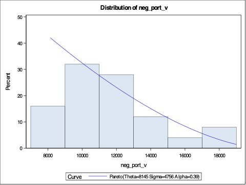 ``` ![](image/3_1b_SAS.png){fig-align="center" width="5in"}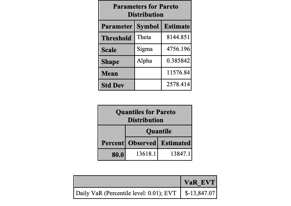 ![](image/3_1c_SAS.png){fig-align="center" width="7in"} Lastly, we use one final `PROC IML` call to calculate the ES using the equation defined above. ```{r} #| eval: false proc iml; title 'EVT Results'; VaR_EVT = &VaR*-1; ES_EVT = ((&VaR + &beta - &xi*&threshold)/(1-&xi))*-1; print "Daily CVaR/ES (Percentile level: &var_percentile); EVT" ES_EVT[format=dollar15.2]; quit; ``` ![](image/3_1d_SAS.png){fig-align="center" width="7in"} ::: These values align with the historical simulation approach that had a much riskier value for VaR and ES compared to the Delta-Normal approach. # VaR Extensions The last section just briefly touches on some of the latest variations and adaptions of the value at risk metric. There are many additions to VaR calculations: - Delta-Gamma VaR - Delta-Gamma Monte Carlo Simulation - Marginal VaR - Incremental VaR - Component VaR Let's discuss each briefly in concept. ::: {.panel-tabset .nav-pills} ## Delta-Gamma VaR The Delta-Gamma approximation approach tries to improve on the Delta-Normal approach by taking into account higher derivatives than the first derivative only. In the expansion of the derivatives we can look at the first two: $$ dV = \frac{\partial V}{\partial RF} \cdot dRF + \frac{1}{2} \cdot \frac{\partial^2 V}{\partial RF^2} + \cdots $$ $$ dV = \Delta \cdot dRF + \frac{1}{2} \cdot \Gamma \cdot dRF^2 $$ Essentially, this approach takes the variance component into account in building the Gamma portion of the equation. Delta-Normal typically **underestimates** VaR when assumptions do not hold. The Delta-Gamma approach tries to correct for this, but it is computationally more intensive. ## Delta-Gamma Monte Carlo The assumption of normality still might not be reliable even with the Delta-Gamma adjustment to Delta-Normal. The Delta-Gamma MC simulation approach simulates the risk factor before using Taylor-series expansion to create simulated movements in the portfolio's value. Just like with regular simulation, the VaR is calculated using the simulated distribution of the portfolio. For a comparison, if you have a large number of things to evaluate in a portfolio with few options, the Delta-Normal approach is fast and efficient enough. However, if you have only a few sources of risk and substantial complexity, the Delta-Gamma approach is better. If you have both a large number of risk factors and substantial complexity, simulation is probably the best approach. ## Marginal VaR The marginal VaR tries to answer the question of how much the VaR will change if we invest one more dollar in a position of the portfolio. In other words, the first derivative of VaR with respect to the weight of a certain position in the portfolio. Assuming normality, this calculation is quite easy: $$ \Delta VaR = \alpha \times \frac{Cov(R_i, R_p)}{\sigma_p} $$ ## Incremental VaR The incremental VaR tries to measure the change in VaR due to the addition of a new position in the portfolio. This is used whenever an institution wants to evaluate the effect of a proposed trade or change in the portfolio of interest. This is slightly different from the marginal VaR that only takes into account an additional dollar of one position instead of adding or subtracting an entire (or multiple) positions. This is trickier to calculate as you now need to calculate the VaR under both portfolios and take their difference. There are Taylor series approximations to his, but they are not as accurate as calculating the full VaR for both portfolios and looking at the difference. ## Component VaR The component VaR decomposes the VaR into its basic components ina way that takes into account the diversification of the portfolio. It is a "partition" of the portfolio VaR that indicates the change of VaR if a given component was deleted. The component VaR is defined in terms of the marginal VaR: $$ VaR_{Comp} = \Delta VaR \times (\$ \text{ value of component}) $$ The sum of all component VaR's is the total portfolio VaR. :::