| Variable | Worst Case | Expected | Best Case |
|---|---|---|---|
| Quantity | 500 | 1,500 | 2,000 |
| Price | $9.00 | $10.00 | $11.00 |
| Variable Cost | $8.00 | $7.00 | $6.50 |
| Fixed Cost | $3,000 | $2,500 | $1,500 |
Introduction to Risk Management
Primer on Risk
Let’s go through a basic example of evaluating risk. Here we have three potential projects to invest in - A, B, or C. The cost of these projects, the expected net return of these projects (profit after subtracting initial costs), and the risk of these projects is defined in the table below:
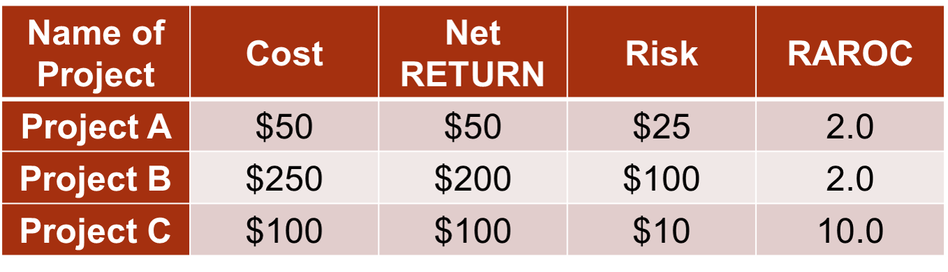
If we evaluate the project based solely on the expected net return we might choose project B. However, project B carries more risk. To combine the information on return and risk we have the Risk Adjusted Return on Capital (RAROC) calculation which is simply the ratio of return to risk. Here we can see that project C is the most return for the risk that we are taking. In fact, investors are not getting paid based on RAROC instead of just return in the investment world. This is because of the incentive problem. Investors were willing to take high risks with other people’s money to make high incomes. They were relying on the government to bail them out if they made a mistake. Now, they are getting paid based on smart investments in terms of both return as well as risk.
However, when evaluating possible scenarios of outcomes, this method of RAROC still falls short. It helps make sound decisions when only considering point estimates of return and risk, but what if that expected return is variable? For example, I want to get in the market of selling widgets. I think I can sell 1500 widgets (quantity, Q) at $10.00 per widget (price, P). It will cost me $7.00 to make each widget (variable cost, VC) and $2,500 to buy the widget making machine (initial / fixed costs, FC). From a basic revenue calculation we can see the net revenue (NR) this enterprise has:
\[ \text{NR} = \text{Q} \times (\text{P}-\text{VC}) - \text{FC} \]
\[ \text{NR} = 1500 \times (10-7) - 2500 \]
\[ \text{NR} = $2,000 \]
Again, this assumes that these inputs are all fixed and known ahead of time. Let’s see what happens when they vary.
Scenario Analysis
In the previous example, we looked at our widget making business and calculated an expected net return of $2,000. If all of the inputs are guaranteed, then we should always invest in this opportunity as it guarantees us a net return that is positive.
Scenario analysis introduces the idea of risk into these calculations. People started accounting for possible extreme values in their estimation of some inputs into calculations. Let’s change the above example slightly. Instead of 1500 widgets being guaranteed to be sold, we have three possibilities. I am most likely to sell 1500 widgets. The best case scenario though is that I can sell 2000 widgets. However, the worst case scenario is that I can only sell 500 widgets. Going through the same net revenue calculation for all three of these possibilities shows some variability to our final result. Now we have an expected net revenue still of $2,000, but with the possibility of making as much as $3,500 and losing as much as $1,000. With those possibilities, the investment is no longer a guarantee. This process can be repeated across all of the variables to see which one has the most impact on the net revenue.
This basic scenario analysis is OK, but still has highly variable outcomes. Is losing money rare or is it more likely that I make some money with a small chance of losing money? We don’t know as only three possibilities are shown. What about interdependence between variables? I imagine that the quantity I sell is highly related to the price that I charge.
Simulation
Simulation analysis allows us to account for all of the possible changes in all these variables and the possible correlation between them. The final output from a simulation analysis is the probability distribution of all possible outcomes. Let’s imagine triangle distributions for the inputs to the above example with the following bounds:
By randomly drawing possible values from the respective triangle distributions 10,000 times and plotting the possible net revenues from each of these simulations we can get a fuller view of the possible outcomes from our widget investment. To do this we use the random.triangular function from numpy in Python to draw values for each input to our equation for a simple demonstration. From there we just calculate the net revenue for each row in our input vectors to get 10,000 different possible net revenues. From there we just plot the corresponding distribution with seaborn.
Code
import numpy as np
import seaborn as sns

sim_size = 10000

Units = np.random.triangular(left = 500, right = 2000, mode = 1500, size = sim_size)
Var_Cost = np.random.triangular(left = 6.5, right = 8, mode = 7, size = sim_size)
Fixed_Cost = np.random.triangular(left = 1500, right = 3000, mode = 2500, size = sim_size)
Price = np.random.triangular(left = 8, right = 11, mode = 10, size = sim_size)

Net_Revenue = (Price - Var_Cost)*Units - Fixed_Cost

ax = sns.histplot(data = Net_Revenue)
ax.set_title('Net Revenue Distribution')
ax.set_xlabel("Dollars")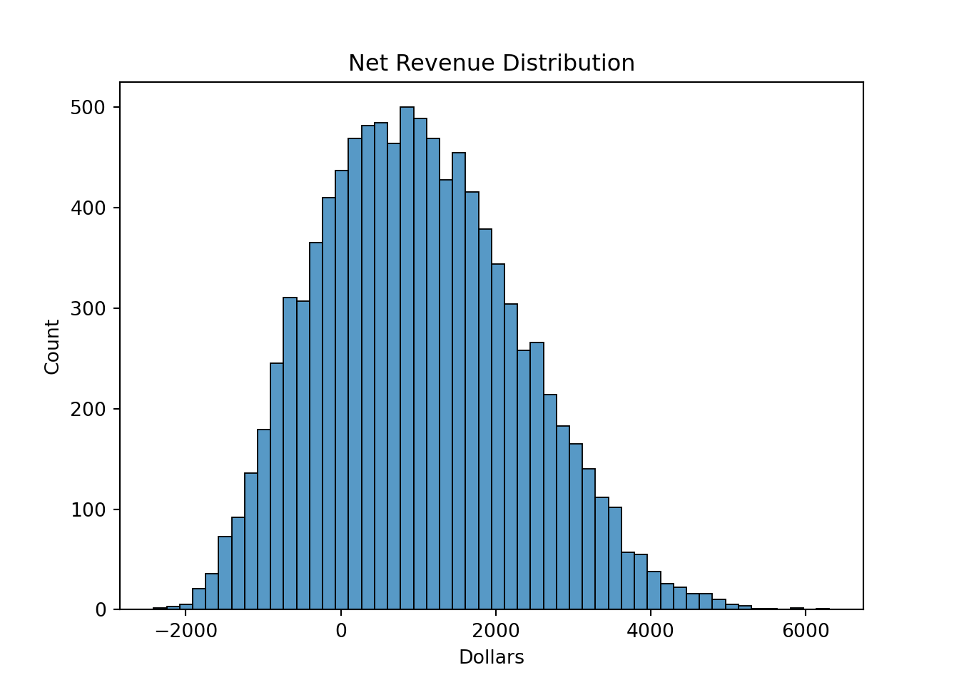
From this we see a much fuller picture of the possible outcomes from our investment. Although the average net revenue is a little over $1,000, in 23.34% of outcomes we lose money. This helps us better evaluate risk. For more information on how to develop simulations like this one, please see the code notes: Introduction to Simulation.
Key Risk Measures
Risk is an uncertainty that affects a system in an unknown fashion and brings great fluctuation in values and outcomes. Remember, that risk is a possible outcome of uncertainty. These outcomes can be measured in a probabilistic sense. Risk has a time horizon and has to be set against a benchmark. Risk analysis uses some of the “typical” statistical measures of spread.
There are some common measures that are used in risk analysis:
Probability of occurrence - measures the probability of risky outcomes like a project losing money, defaulting on a loan, downgrading of a company, etc.
Standard deviation / variance - measures spread in a two-sided manner that works best in normality or symmetric distributions.
Semi-standard deviation - measures of dispersion for the values falling on the risk side of a distribution. For example, if you were measuring risk for profit the semi-standard deviation is calculated as:
\[ \sigma_{semi} = \sqrt{\frac{1}{T} \sum_{t=1}^T \min(X_t - \bar{X}, 0)^2} \]
Volatility - measures the standard deviation of an asset’s logarithmic returns as follows:
\[ \sigma_{volatility} = \sqrt{\frac{1}{T} \sum_{t=1}^T \log(\frac{X_t}{X_{t-1}})^2} \]
Value at Risk (VaR) - measures the amount of money at risk given a particular time period at a particular probability of loss. For example, a 1 year 1% VaR being $10,000 means there is a 1% chance you will lose more than $10,000 in 1 year.
Expected Shortfall (ES) - measures the average money in the worst % of cases given a particular period of time. For example, in the worst 1% of scenarios, the average amount of money you will lose in one year is $15,000.
Value at risk and expected shortfall are some of the most popular measures of risk so we will discuss them in much further detail throughout these notes.
Value at Risk (VaR)
Value at risk (VaR) was developed in the early 1990’s by JP Morgan. They were made famous in JP Morgan’s “4:15pm” report which was a daily report given to the Chief Risk Officer at JP Morgan detailing the risk of all current investments / portfolios. In 1994, JP Morgan launched RiskMetrics®. VaR has been widely used since that time and people are researching other similar measures.
The VaR calculation is aimed at making a statement of the following form: We are 1% certain that we will lose more than $10,000 in the next 3 days. VaR is the maximum amount at risk to be lost over a period of time and at a particular level of confidence. Essentially, VaR is associated with a percentile (quantile) of a distribution as shown in the chart below:
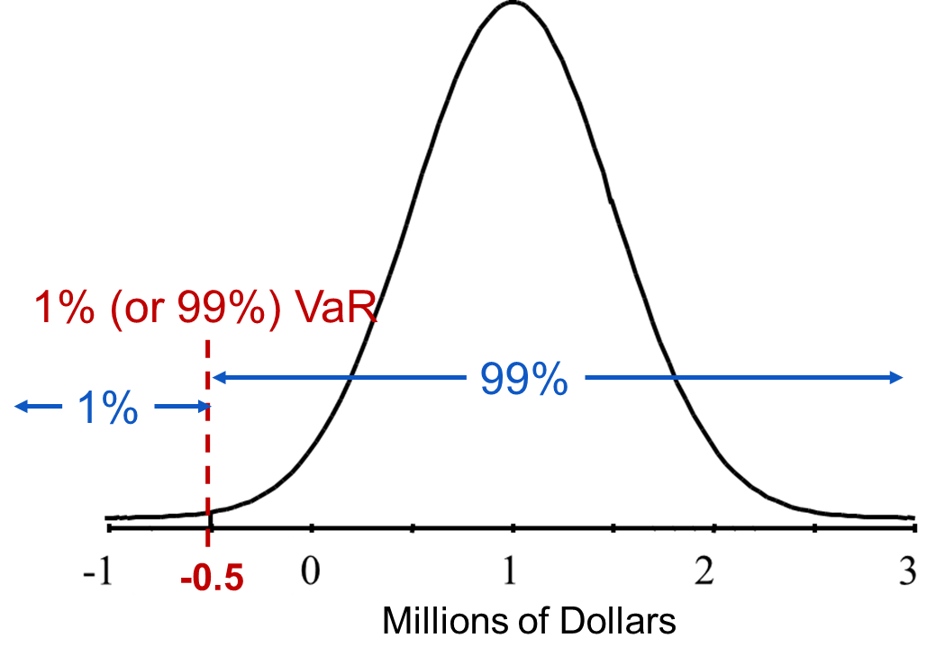
For the plot above, the one year 1% VaR is $500,000. In other words, there is a 1% chance you will lose at least $500,000 by holding that portfolio for a year. Although most of the portfolio value over the next year is positive with the average being one million in value, there is some risk. VaR calculates the value that is most at risk in terms of a quantile. For costs, the VaR would be on the high end since risk is high cost, not low cost.
The main steps to estimating VaR are the following:
Identify the variable of interest (asset value, portfolio value, credit losses, insurance claims, etc.)
Identify the key risk factors that impact the variable of interest (asset prices, interest rates, duration, volatility, default probabilities, etc.)
Perform deviations in the risk factors to calculate the impact in the variable of interest
The main question is how to estimate the distribution that we will calculate the quantile of. There are three main approaches to estimating the distribution in VaR:
Delta-Normal (Variance-Covariance) Approach
Historical Simulation Approach(s)
Simulation Approach
These will be discussed in later sections of these notes.
Expected Shortfall (ES)
There are some downsides to value at risk as a calculation. One of them is that VaR ignores the distribution of a portfolio’s return beyond its VaR value. For example, if two portfolios each have a one year 1% VaR of $100,000, does that mean you are indifferent between the two? What if you then knew the maximum loss for one of the portfolios is $250,000, while the other has a maximum loss of $950,000. VaR ignores the magnitude of the worst outcomes. Another downside of VaR is that under non-normality, VaR may not capture diversification. Mathematically, it fails to satisfy the subadditivity property:
\[ \text{Risk(A + B)} \le \text{Risk(A)} + \text{Risk(B)} \]
The VaR of a portfolio with two securities may be larger than the sum of the VaR’s of the securities in the portfolio.
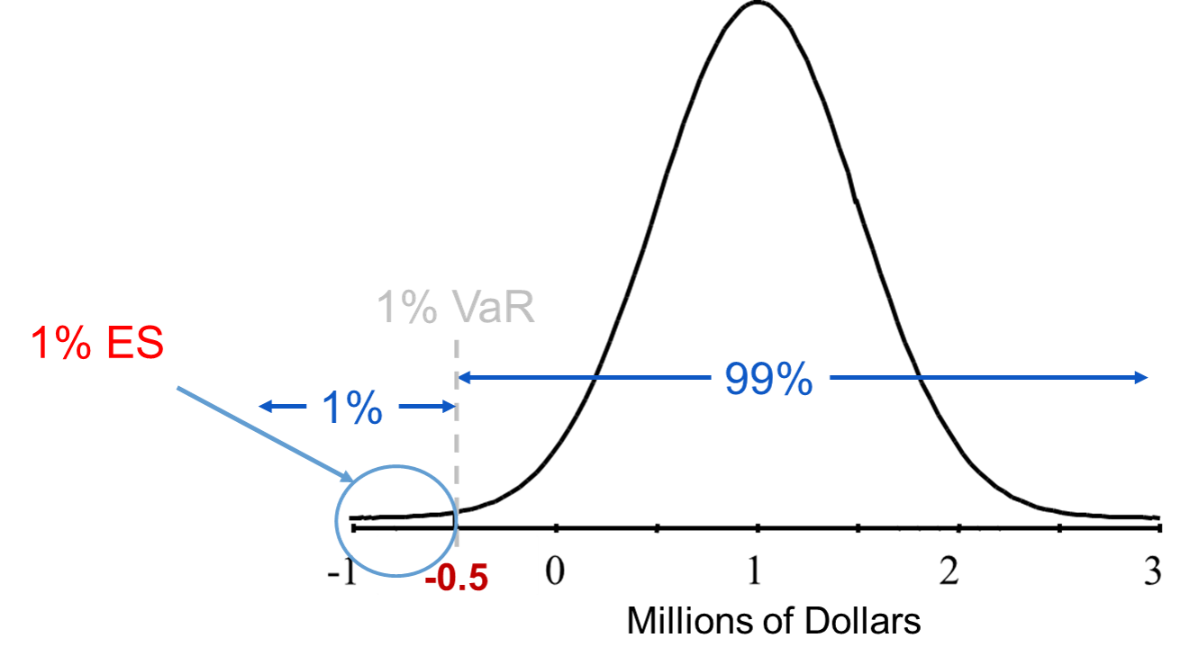
The expected shortfall (ES) (also called the conditional value at risk (CVaR)) is a measure that doesn’t have the two drawbacks described above. Given a confidence level and a time horizon, a portfolio’s ES is the expected loss one suffers given that a “bad” event occurs. The ES is a conditional expectation that tries to answer what you should expect to lose if your loss exceeds the VaR. It is the expected (average) value of the portfolio in the circled region below:
The main question is how to estimate the distribution that we will calculate the average of the worst case outcomes. There are three main approaches to estimating the distribution in ES and they are the same as VaR:
Delta-Normal (Variance-Covariance) Approach
Historical Simulation Approach(s)
Simulation Approach
These will be discussed in later sections of these notes.
Returns
Before getting into detail on calculating the distributions behind VaR and ES, let’s briefly talk about returns. A lot of the calculations in the remaining pieces of this document will revolve around calculating returns on assets. There are two main methods for calculating returns:
Arithmetic returns
Geometric returns
As we detail the differences between these approaches, here is the notation we will use:
Arithmetic Returns (\(r_t\)) - return at a period \(t\) (value of holding an asset from period \(t-1\) to period \(t\))
Price (\(P_t\)) - price at a given time period \(t\)
Lag Price (\(P_{t-1}\)) - price at a given time period \(t-1\)
Dividend (\(D_t\)) = sum of money regularly paid from company to shareholders at time period \(t\). For small time periods we typically ignore dividends (set them equal to 0). Equivalently, we can think about the price of an asset where dividends are fully reinvested and reflected in the price itself.
Arithmetic returns are calculated as follows:
\[ r_t = \frac{P_t + D_t - P_{t-1}}{P_{t-1}} = \frac{P_t - P_{t-1}}{P_{t-1}} \text{ when } D_t = 0 \]
If \(r_1 = 5\%\) and \(r_2 = -5\%\), what is the total return of the two days? It is not 0%! This is how we would get the return, \(r_{0,2}\), over the two days:
\[ r_{0,2} = \frac{P_2 - P_0}{P_0} = \cdots = \frac{P_1}{P_0}r_2 + r_1 \ne r_2 + r_1 \]
For example, if we had $100 that we got 5% return on after 1 year, but lost 5% in year two with arithmetic returns we would have:
\[ P_0 = 100, P_1 = 100 \times (1 + 0.05) = 105, P_2 = 105 \times (1 - 0.05) = 99.75 \]
\[ r_{0,2} = \frac{99.75 - 100}{100} = -0.25\% \]
Geometric returns (denoted \(R_t\) instead) on the other hand are calculated as follows:
\[ R_t = \log(\frac{P_t + D_t}{P_{t-1}}) = \log(\frac{P_t}{P_{t-1}}) = \log(P_t) - \log(P_{t-1}) \text{ when } D_t = 0 \]
If \(R_1 = 5\%\) and \(R_2 = -5\%\), what is the total return of the two days? It is 0%! This is how we would get the return, \(R_{0,2}\), over the two days:
\[ R_{0,2} = \log(\frac{P_2}{P_0}) = \log(\frac{P_2}{P_1} \times \frac{P_1}{P_0}) = \log(\frac{P_2}{P_1}) + \log(\frac{P_1}{P_0}) = R_1 + R_2 \]
Lets use the previous example’s prices to see what the geometric returns would be:
\[ P_0 = 100, P_1 = 105, P_2 = 99.75 \]
\[ R_1 = 4.88\% \]
\[ R_{0,2} = \frac{99.75}{100} -4.88\% \]
The difference between arithmetic and geometric means is very small when returns are close to zero. We can see this by expanding the natural log:
\[ R_t = \log(\frac{P_t}{P_{t-1}}) = \log(\frac{P_t - P_{t-1}}{P_{t-1}} + 1) = \log(1 + r_t) = r_t - \frac{r_t^2}{2} + \frac{r_t^3}{3} - \cdots \]
This is approximately \(r_t\) when \(r_t\) is small. The following are the arithmetic returns and geometric returns for Alphabet Inc in early 2025:
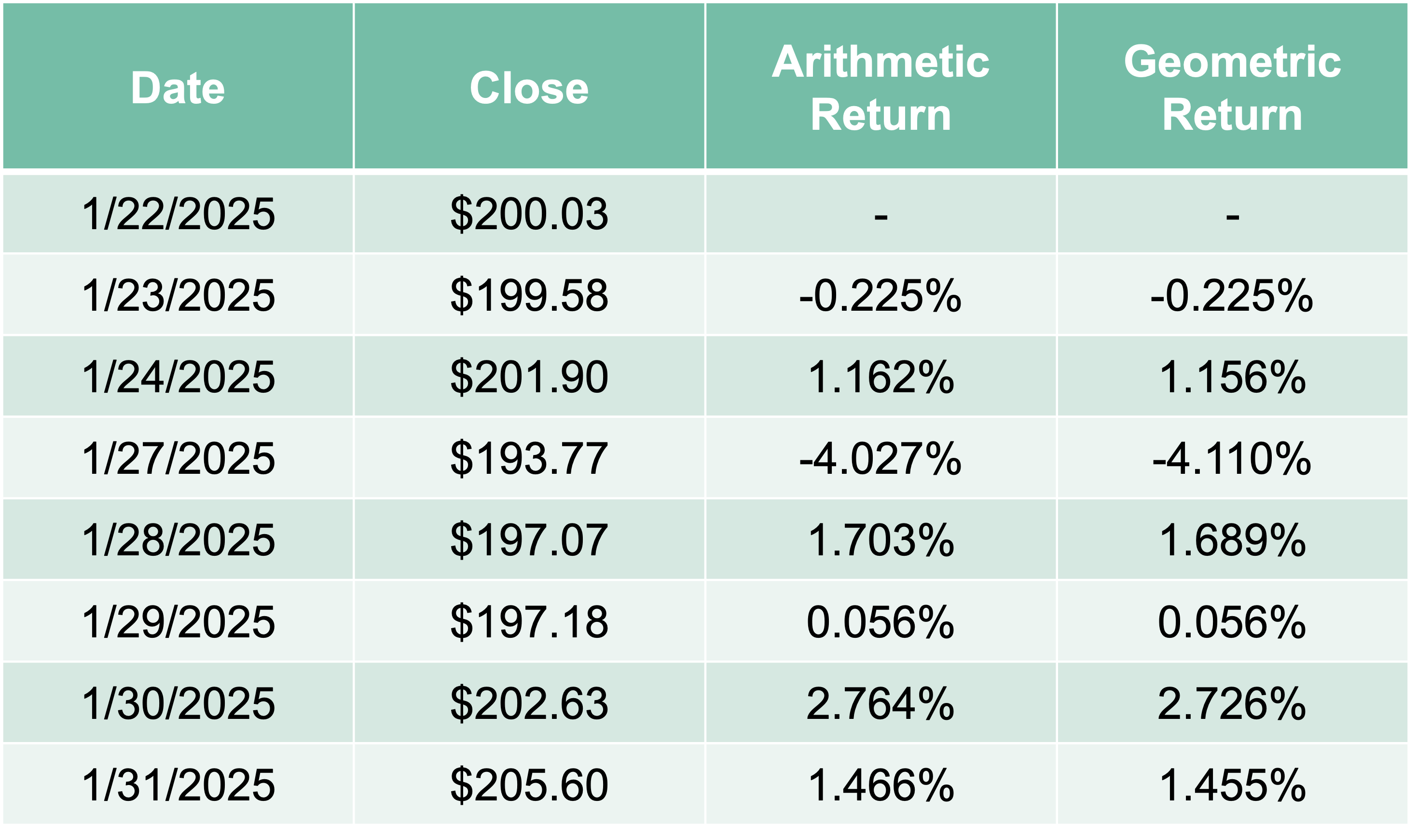
As you can see above, the two different types of returns are approximately equal.