Code
library(quantmod)

tickers = c("AAPL", "MSFT")

getSymbols(tickers)
[1] "AAPL" "MSFT"The main steps to estimating VaR and ES are the following:
Identify the variable of interest (asset value, portfolio value, credit losses, insurance claims, etc.)
Identify the key risk factors that impact the variable of interest (asset prices, interest rates, duration, volatility, default probabilities, etc.)
Perform deviations in the risk factors to calculate the impact on the variable of interest
The main question is how to estimate the distribution that we will calculate the quantile of. There are three main approaches to estimating the distribution in VaR:
Delta-Normal (Variance-Covariance) Approach
Historical Simulation Approach(es)
Simulation Approach
First we will discuss how to do this for value at risk followed by expected shortfall.
The Delta Normal approach has two key characteristics that define it. First, we will discuss the Normal part of the name. Suppose that the value, \(V\), of an asset is a function of a normally distributed risk factor, \(RF\). Assume that the relationship between this risk factor and the value of the asset is linear:
\[ V = \beta_0 + \beta_1 RF \]
In this situation it is easy to calculate the VaR. If \(RF\) is normally distributed in the above equation, then \(V\) would also be normally distributed as well. The 2.5% VaR on any normal distribution is the quantile shown below:
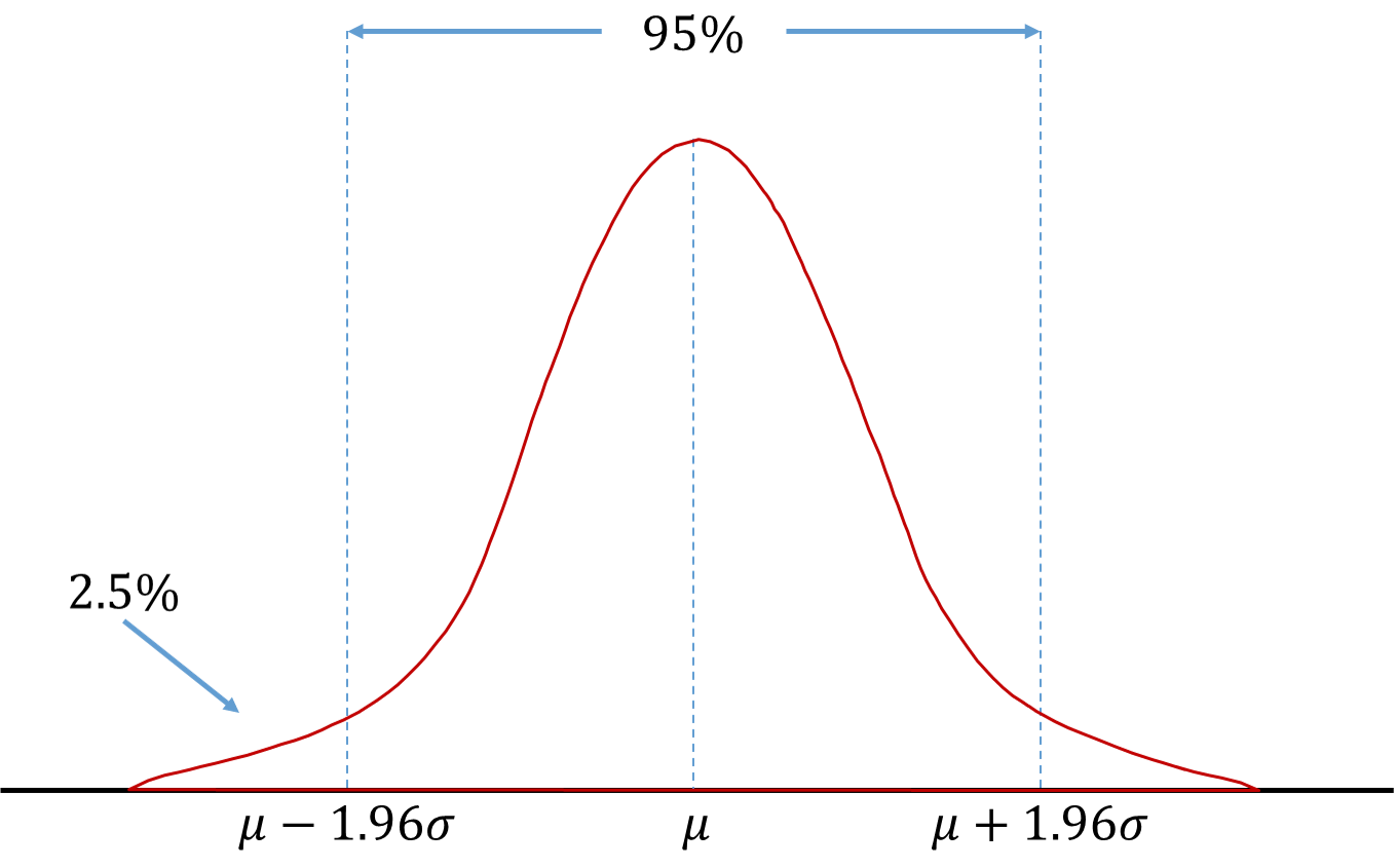
The VaR at 2.5% is just \(\mu - 1.96\sigma\). With an estimate of \(\mu\) and \(\sigma\) we can estimate this number easily. In fact, any VaR for a normal distribution can be calculated by adjusting the 1.96 to match the quantile of interest. For example, the 1% VaR is \(\mu - 2.33\sigma\).
The above approach works great if the relationship is linear between \(RF\) and \(V\). What if the relationship between the two is nonlinear:
\[ V = \beta_0 + \beta_1 RF^2 \]
Finding the extreme of a normally distributed value and squaring that value does not equal the extreme value for a squared risk factor. However, we can still use the normality assumption to help calculate the VaR.
This is where the delta piece of the name comes into play. The derivative of the relationship will help us approximate what we need. Remember, the derivative at a specific point (say \(RF_0\)) is the tangent line at that point. If we zoom in closer to the area around \(RF_0\) the relationship is approximately linear as seen below:

Small changes of the risk factor result in small changes of the value of the asset. We can approximate these small changes with the slope. We can see this more mathematically by looking at the Taylor-series expansion of a function’s derivatives:
\[ dV = \frac{\partial V}{\partial RF} \cdot dRF + \frac{1}{2} \cdot \frac{\partial^2 V}{\partial RF^2} \cdot dRF^2 + \cdots \]
The Delta-Normal approach assumes that only the first derivative is actually important. We can evaluate this first derivative at a specific point \(RF_0\) which is typically some initial value:
\[ dV = \frac{\partial V}{\partial RF} \Bigg|_{RF_0} \cdot dRF \rightarrow \Delta V = \delta_0 \cdot \Delta RF \]
The change in the value of the asset / portfolio is a constant (\(\delta_0\)) multiplied by the change in the risk factor. This is a linear relationship between the changes. All we need to know is the distribution of \(\Delta RF\). Luckily, we already assumed normality for \(RF\). Since \(\Delta RF = RF_t - RF_{t-1}\) and each of \(RF_t\) and \(RF_{t-1}\) are normal, then \(\Delta RF\) is normally distributed since the difference in normal distributions is still normal. Therefore, the change in the value of the asset / portfolio, \(\Delta V\) is also normally distributed by the same logic. Since \(\Delta V\) is normally distributed we can easily calculate any VaR values for the change in the portfolio as we did above.
Let’s work through an example! Suppose that the variable of interest is a portfolio consisting of \(N\) units in a certain stock, \(S\). The price of the stock at time \(t\) is denoted as \(P_t\). Therefore, the value of the portfolio is \(N \times P_t\). Let’s assume that the price of the stock follows a random walk:
\[ P_t = P_{t-1} + \varepsilon_t \]
with \(\varepsilon_t\) following a normal distribution with mean 0 and standard deviation \(\sigma\). Therefore, the change in the value of the portfolio is \(N \times \Delta P_t\) with \(\Delta P_t = P_t - P_{t-1} = \varepsilon_t\) which is a normal distribution. We can then look up the VaR for a portfolio under this structure by just looking up the corresponding point on the normal distribution. If we wanted the 1% VaR for the change in the value of the portfolio, it would just be \(0 - 2.33\sigma\). This is why the Delta-Normal approach is sometimes referred to as the variance-covariance approach. If you know the variances of your data and are willing to assume normality, then the calculation of the VaR is rather straight forward.
Let’s put some numbers to the previous example. Suppose you invested $100,000 in Apple today (bought Apply stock). Historically, the daily standard deviation of Apple returns are 1.36%. Let’s also assume daily returns for Apple have a mean return of 0.1%. Let’s assume that the returns for Apple follow a normal distribution. Then the 1 day, 1% VaR is calculated as \(\$100,000 \times (0.001 + (-2.33) \times 0.0181 ) = -\$3,263.83\). In other words, you think there is a 1% chance of losing more than $3,263.83 by holding that portfolio of Apple stock for a single day.
What if we had two assets in our portfolio? Luckily, these calculations are still easily worked out under the assumption of normality. If we had two random variables X and Y that were both normally distributed, then the variance of a linear combination of X and Y, \(aX + bY\) would be the following:
\[ \sigma^2 = a^2 \sigma_x^2 + b^2 \sigma_Y^2 + 2ab \times Cov(X, Y) \]
Suppose you invested $200,000 in Microsoft and $100,000 in Apple. Assume the historical daily average return is 0.1% for both. Also assume that the historical standard deviation of daily returns for Microsoft and Apple are 1.40% and 1.36% respectively. Lastly, assume that the historical correlation between the two returns is 0.488. Under the assumption that both returns follow normal distributions then the variance of that portfolio is the following:
\[ \sigma_P^2 = (2/3)^2 \sigma_M^2 + (1/3)^2 \sigma_A^2 + 2(2/3)(1/3) \times Cov(A, M) \]
\[ \sigma_P^2 = (2/3)^2 0.0140^2 + (1/3)^2 0.0136^2 + 2(2/3)(1/3) \times (0.488 \times 0.0140 \times 0.0136) = 0.00015 \]
Then the one day, 1% VaR for this portfolio is \(\$300,000 \times (0.001 + (-2.32635) \times \sqrt{0.00015} ) = -\$8,814.43\).
Let’s see how we can do this in each of our software!
It is easy to replicate the calculations we did above by hand using R. First, we need to collect our stock data. We can do this using the getSymbols function. The input to the getSymbols function is the stock tickers from the New York Stock Exchange accessed through Yahoo Finance ®. It will pull all daily opening, closing, high, and low prices for the given stock tickers and save them in data frames under the same names. The last function will extract only the last number of observations from the data sets. Here we are looking at the last 500 days. Every day you run this code, the last 500 days will change so the calculations could be different. Specifically we are looking only at the adjusted closing prices for each stock. The ROC function will give us the daily returns for each of these stocks now saved as the variables msft_r and appl_r.
library(quantmod)
tickers = c("AAPL", "MSFT")
getSymbols(tickers)[1] "AAPL" "MSFT"stocks <- cbind(last(AAPL[,6], '500 days'), last(MSFT[,6], '500 days'))
stocks$msft_r <- ROC(stocks$MSFT.Adjusted)
stocks$aapl_r <- ROC(stocks$AAPL.Adjusted)
head(stocks) AAPL.Adjusted MSFT.Adjusted msft_r aapl_r
2023-02-09 149.3000 259.3635 NA NA
2023-02-10 149.6667 258.8520 -0.001974338 0.002453317
2023-02-13 152.4814 266.9392 0.030764753 0.018632184
2023-02-14 151.8372 267.7755 0.003128039 -0.004233998
2023-02-15 153.9483 265.6352 -0.008025077 0.013807833
2023-02-16 152.3427 258.5633 -0.026983632 -0.010484485Next, we just calculate the historical numbers we need for our calculations, namely the correlation between and the variance of the stocks. Instead of the correlation, we could also use the covariance directly. The cov, var, and cor functions give us the covariance, variances, and correlations respectively. From there we just recreate the equation written above in code. Lastly, we use the qnorm function to get the quantile from the normal distribution for our VaR calculation.
library(scales)

var.msft <- var(stocks$msft_r, na.rm=TRUE)
var.aapl <- var(stocks$aapl_r, na.rm=TRUE)
cov.m.a <- cov(stocks$msft_r, stocks$aapl_r, use="pairwise.complete.obs")
cor.m.a <- cor(stocks$msft_r, stocks$aapl_r, use="pairwise.complete.obs")

VaR.percentile = 0.01
AAPL.inv <- 100000
MSFT.inv <- 200000

var.port <- (MSFT.inv/(MSFT.inv+AAPL.inv))^2*var.msft + (AAPL.inv/(MSFT.inv+AAPL.inv))^2*var.aapl + 2*(AAPL.inv/(MSFT.inv+AAPL.inv))*(MSFT.inv/(MSFT.inv+AAPL.inv))*cov.m.a

VaR.DN.port <- (AAPL.inv+MSFT.inv)*qnorm(VaR.percentile)*sqrt(var.port)
dollar(VaR.DN.port)
[1] "-$8,530.90"If the number above is different than the number we calculated by hand, then it is simply a result of a different time period and different data underlying it. The code is written to always use the most up to date data for each stock.
Another great aspect of the VaR under the normality assumption is the ease of calculating any \(n\)-day VaR from the 1-day VaR. This is defined simply as \(VaR_n = \sqrt{n} \times VaR_1\). Another great reason why the normality assumption in the Delta-Normal approach makes the calculation of VaR numbers rather easy.
First, we need to collect historical stock data. We can do this through the yfinance package in Python. By putting in the stock ticker as it appears in the New York Stock Exchange, we can pull data from Yahoo Finance ® through this function. The download function then gets us historical, daily opening prices, closing prices, high prices, and low prices. We will grab data all the way back to 2007. We want to calculate the daily return on the closing prices. We can use the pct_change() function to calculate the percentage change. Next, we just calculate the historical numbers we need for our calculations, namely the correlation between and the variance of the stocks. Instead of the correlation, we could also use the covariance directly. The cov and corrcoef functions from numpy give us the covariance and variances as well as the correlations respectively. From there we just recreate the equation written above in code. Lastly, we use the norm.ppf function from scipy.stats to get the quantile from the normal distribution for our VaR calculation.
import yfinance as yf

stocks = yf.download("AAPL MSFT", start = "2007-01-01", group_by='tickers')
[                       0%                       ]
[*********************100%***********************] 2 of 2 completedstocks = stocks.tail(500)
stocks['msft_r'] = stocks['MSFT'].pct_change()['Close']
stocks['aapl_r'] = stocks['AAPL'].pct_change()['Close']
stocks.head(5)Ticker MSFT ... AAPL msft_r aapl_r
Price Open High Low ... Volume
Date ...
2023-02-10 257.307301 259.825965 256.451353 ... 57450700 NaN NaN
2023-02-13 263.318664 270.166279 262.836556 ... 62199000 0.031243 0.018807
2023-02-14 268.267440 270.530291 264.932161 ... 61707600 0.003133 -0.004225
2023-02-15 264.648875 267.025905 262.538140 ... 65573800 -0.007993 0.013903
2023-02-16 260.407704 263.090490 258.316714 ... 68167900 -0.026623 -0.010429
[5 rows x 12 columns]import numpy as np
import scipy.stats as sps
import locale
var_msft = np.cov(np.array([stocks['msft_r'][1:], stocks['aapl_r'][1:]]))[0,0]
var_aapl = np.cov(np.array([stocks['msft_r'][1:], stocks['aapl_r'][1:]]))[1,1]
cov_m_a = np.cov(np.array([stocks['msft_r'][1:], stocks['aapl_r'][1:]]))[0,1]
cor_m_a = np.corrcoef(np.array([stocks['msft_r'][1:], stocks['aapl_r'][1:]]))[0,1]
VaR_percentile = 0.01
AAPL_inv = 100000
MSFT_inv = 200000
var_port = (MSFT_inv / (MSFT_inv + AAPL_inv))**2*var_msft + (AAPL_inv/(MSFT_inv+AAPL_inv))**2*var_aapl + 2*(AAPL_inv/(MSFT_inv+AAPL_inv))*(MSFT_inv/(MSFT_inv+AAPL_inv))*cov_m_a
VaR_DN_port = (AAPL_inv+MSFT_inv)*sps.norm.ppf(VaR_percentile)*np.sqrt(var_port)
locale.currency(VaR_DN_port, grouping = True)'-$8,542.70'If the number above is different than the number we calculated by hand, then it is simply a result of a different time period and different data underlying it. The code is written to always use the most up to date data for each stock.
Another great aspect of the VaR under the normality assumption is the ease of calculating any \(n\)-day VaR from the 1-day VaR. This is defined simply as \(VaR_n = \sqrt{n} \times VaR_1\). Another great reason why the normality assumption in the Delta-Normal approach makes the calculation of VaR numbers rather easy.
We will use the functions in the R section of the code to get the necessary data in a data set called stocks. First, we will use PROC CORR to get us the necessary information on the variances, covariances, and correlations. You could easily just write these numbers down, but we are going to use the out = option to store the needed information into a data set called covar_results. We then use the DATA step to create MACRO variables that store the values of the covariance between and variances of the stocks.
proc corr data=SimRisk.stocks cov out=covar_results plots;
    var msft_r aapl_r;
run;

data _null_;
    set covar_results(where = (_type_ eq 'COV'));
    if upcase(_name_) eq 'MSFT_R' then do;
        call symput("var_msft",msft_r);
        call symput("covar",aapl_r);
    end;
    if upcase(_name_) eq 'AAPL_R' then do;
        call symput("var_aapl",aapl_r);
    end;
run;

data _null_;
    set covar_results(where = (_type_ eq 'CORR'));
    if upcase(_name_) eq 'MSFT_R' then do;
        call symput("corr",aapl_r);
    end;
run;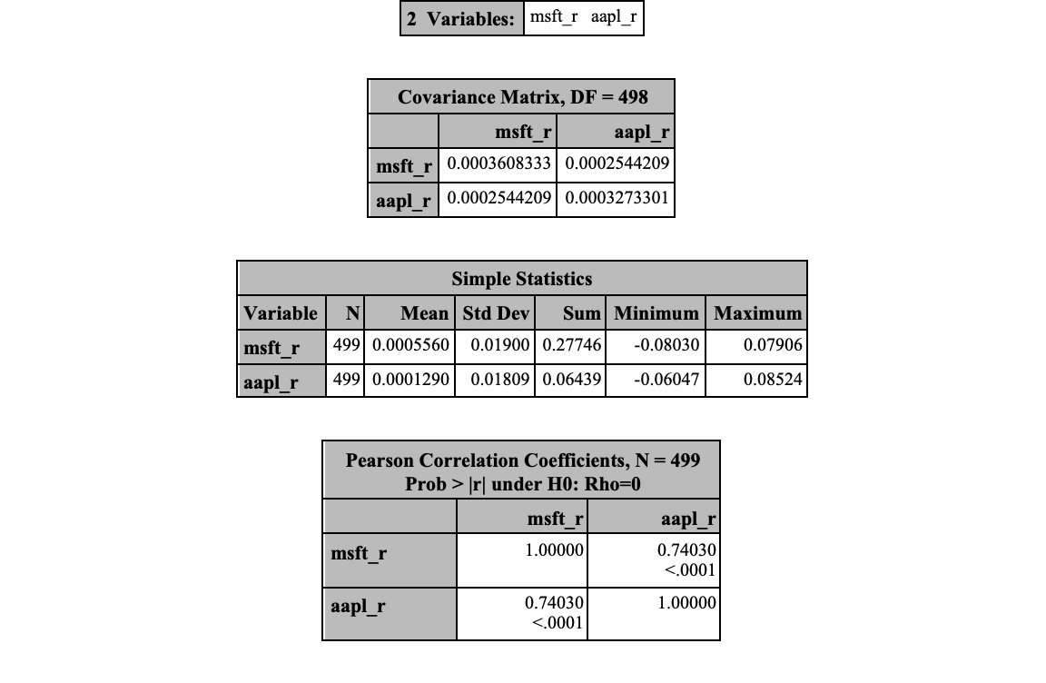
Next, we need to use PROC IML to do the calculations by hand. PROC IML is the interactive matrix language of SAS. It is similar in design to R. We start by defining some MACRO variables for the amount we invested in each stock as well as the desired VaR percentile. From there we invoke PROC IML and put in calculations as we would in R. We print out the results of these equations that we defined above.
%let msft_position = 200000;
%let aapl_position = 100000;
%let var_percentile = 0.01;

proc iml;
title 'VaR Results';

msft_p_weight = &msft_position/(&msft_position + &aapl_position);
aapl_p_weight = &aapl_position/(&msft_position + &aapl_position);

P_variance =  &var_msft*(msft_p_weight)**2 + &var_aapl*(aapl_p_weight)**2
                   + 2*aapl_p_weight*msft_p_weight*&covar;
P_StdDev=sqrt(P_variance);

VaR_normal = (&msft_position + &aapl_position)*PROBIT(&var_percentile)*SQRT(P_variance);

print "Daily VaR (Percentile level: &var_percentile); Delta-Normal" VaR_normal[format=dollar15.2];

quit;
If the number above is different than the number we calculated by hand, then it is simply a result of a different time period and different data underlying it.
Another great aspect of the VaR under the normality assumption is the ease of calculating any \(n\)-day VaR from the 1-day VaR. This is defined simply as \(VaR_n = \sqrt{n} \times VaR_1\). Another great reason why the normality assumption in the Delta-Normal approach makes the calculation of VaR numbers rather easy.
The historical simulation approach is a non-parametric (distribution free) approach to estimating the VaR and ES values. This approach, as the name states, depends solely on historical data. For example, if history suggests that only 1% of the time Apple’s daily returns were below -4%, then the 1% VaR for daily returns is just -4%. Essentially, we just find the quantiles of our historical data! Let’s work through some examples.
Suppose you invested $100,000 in Apple today. You have 500 historical observations on Apple’s daily returns. You want to compute the daily, 1% VaR of your portfolio. All we have to do is find the 1% quantile of our 500 observations. To do this we simply calculate the portfolio’s value as if the 500 historical observations we had were possible future values of the Apple’s daily returns. We sort these 500 portfolio values from worst to best. The 1% of 500 days is 5 days, so we need to find a loss that is only exceeded 5 times. In other words, the 1% VaR would be the 6th observation in our sorted possible portfolio values as shown below:
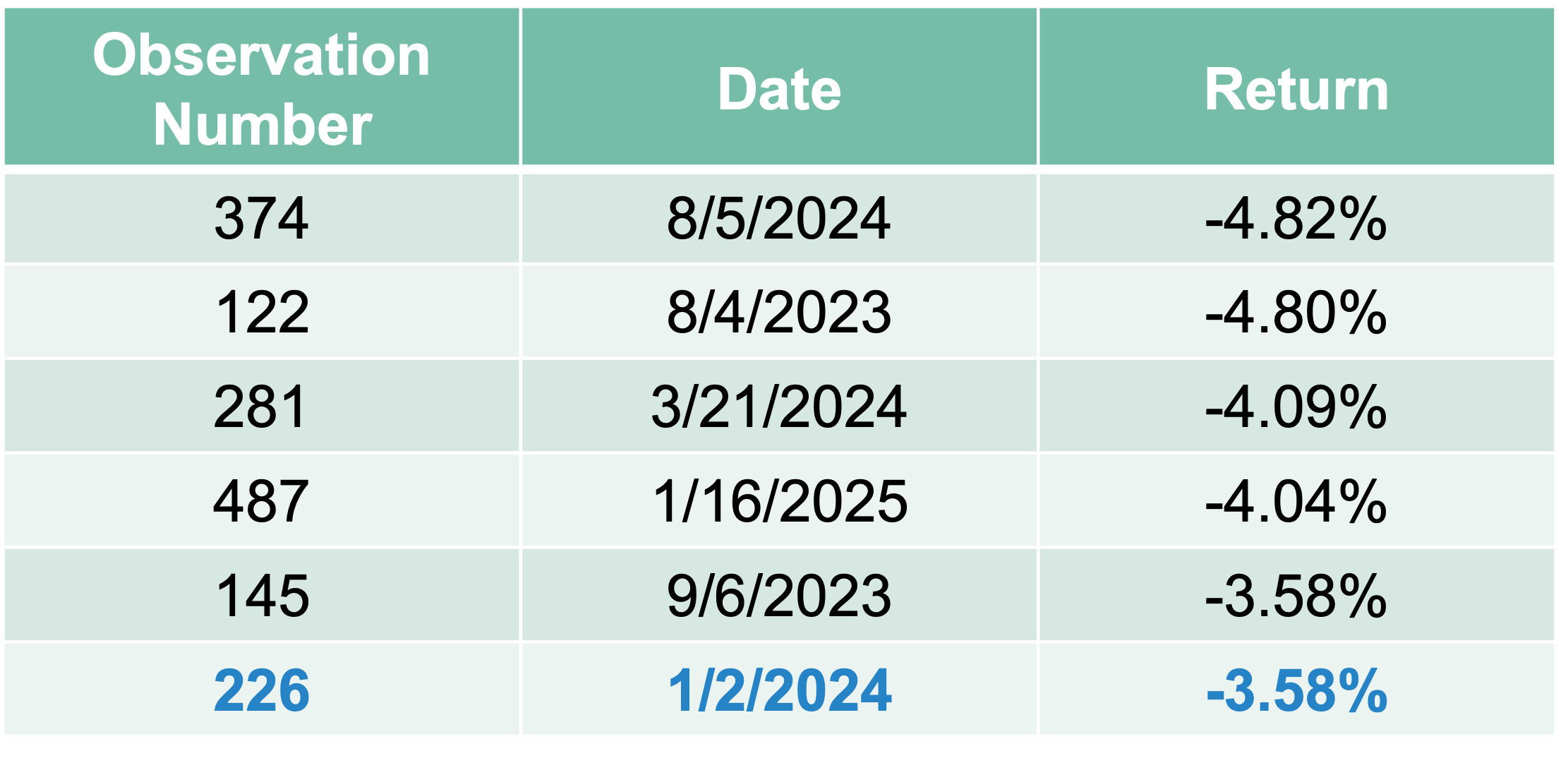
Here we can see that our portfolio dropping 3.58% in value is the 6th worst occurrence.
Let’s see how to do this in each of our software!
It is rather easy to sort data in R. We simply use the order function inside of the [] to resort the rows of the variable of interest. We then just use the head function to define which elements we want to look at. Here we want the 6th element.
VaR.H.AAPL <- AAPL.inv*stocks$aapl_r[head(order(stocks$aapl_r), 6)[6]]
print(VaR.H.AAPL)
aapl_r
2024-01-02 -3644.261It is rather easy to sort data in Python. We simply use the sort.values() function to resort the rows of the variable of interest. We then just use the [] to define which elements we want to look at. Here we want the 6th element (5 in Python because it starts at 0).
VaR_H_AAPL = AAPL_inv * stocks['aapl_r'].sort_values()[5]<string>:1: FutureWarning: Series.__getitem__ treating keys as positions is deprecated. In a future version, integer keys will always be treated as labels (consistent with DataFrame behavior). To access a value by position, use `ser.iloc[pos]`locale.currency(VaR_H_AAPL, grouping = True)'-$3,578.67'We will use PROC IML again to easily calculate this quantile in SAS. Again, we will read in our data that we obtained from R. We then calculate the portfolio values as we did before. Lastly, we just use the SORT function from the CALL statement to sort these returns. From there we just use the 6th observation.
proc iml;

use SimRisk.stocks var {aapl_r};
read all var _all_ into returns;

portfolio_return = &aapl_position*returns[,1];

call sort(portfolio_return,{1});
number_of_observations = nrow(portfolio_return);

VaR_historical = portfolio_return[6,1];

print "Daily VaR (Percentile level: &var_percentile); Historical" VaR_historical[format=dollar15.2];

title;
quit;
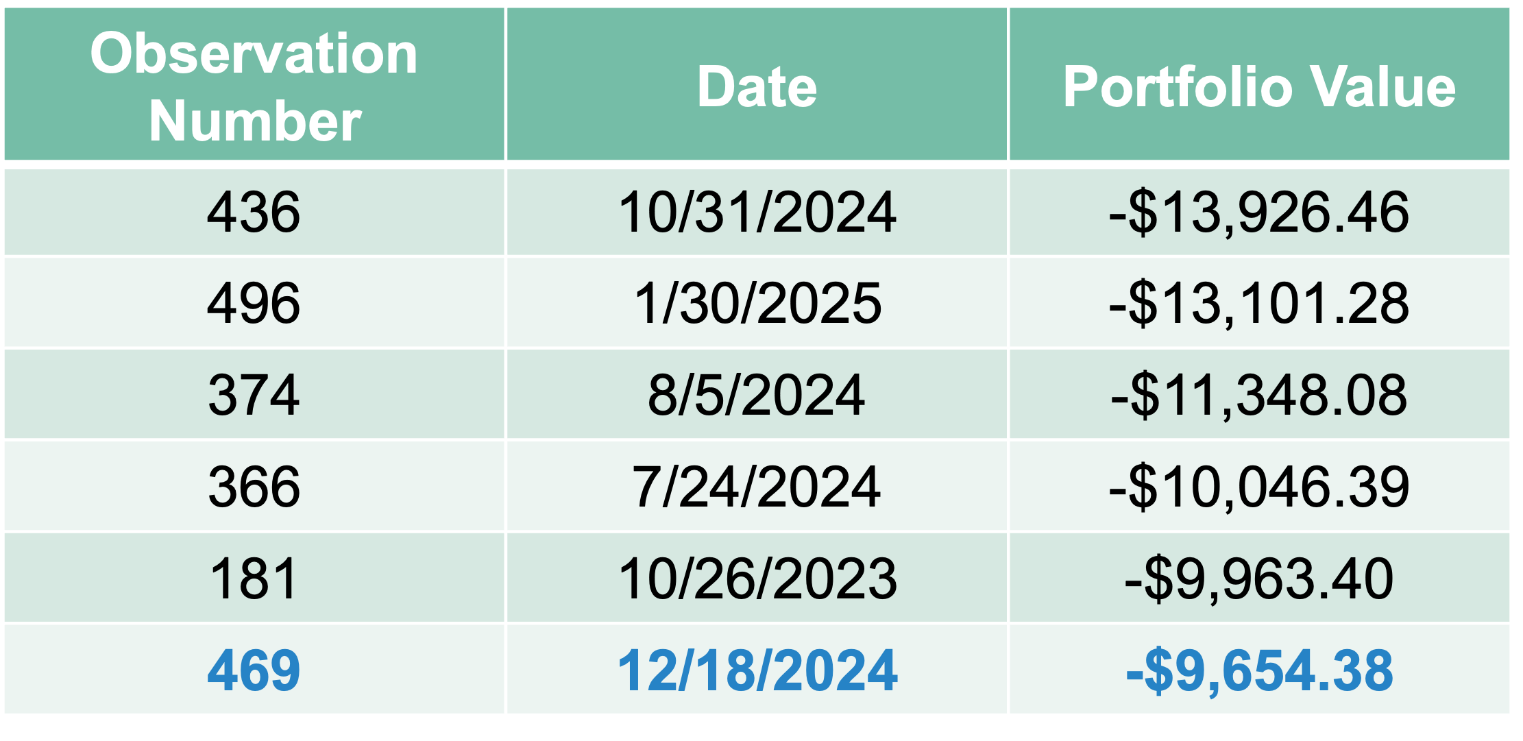
We can easily extend this to a two position portfolio example by taking the same approaches. Suppose you invested $200,000 in Microsoft and $100,000 in Apple today. You have 500 historical observations on both returns. Simply calculate the portfolio’s value as if each of the previous 500 days is a possible scenario for your one day return on this portfolio. We then sort these 500 possible scenarios and the 1% VaR will be the 6th observation as shown below:
Let’s see how to do this in each of our software!
Just like with the one position portfolio, it is rather easy to sort data in R. We simply use the order function inside of the [] to resort the rows of the variable of interest. We then just use the head function to define which elements we want to look at. Here we want the 6th element.
stocks$port_v <- MSFT.inv*stocks$msft_r + AAPL.inv*stocks$aapl_r

VaR.H.port <- stocks$port_v[order(stocks$port_v)[6]]
dollar(as.numeric(VaR.H.port))
[1] "-$9,822.38"Just like with the one position portfolio, it is rather easy to sort data in Python. We simply use the sort.values() function to resort the rows of the variable of interest. We then just use the [] to define which elements we want to look at. Here we want the 6th element.
stocks['port_v'] = MSFT_inv*stocks['msft_r'] + AAPL_inv*stocks['aapl_r']

VaR_H_port = stocks['port_v'].sort_values()[5]
<string>:2: FutureWarning: Series.__getitem__ treating keys as positions is deprecated. In a future version, integer keys will always be treated as labels (consistent with DataFrame behavior). To access a value by position, use `ser.iloc[pos]`locale.currency(VaR_H_port, grouping = True)'-$9,654.38'Just like with the one position portfolio, we will use PROC IML again to easily calculate this quantile in SAS. Again, we will read in our data that we obtained from R. We then calculate the portfolio values as we did before. Lastly, we just use the SORT function from the CALL statement to sort these returns. From there we just use the 6th observation.
proc iml;

use SimRisk.stocks var {msft_r aapl_r};
read all var _all_ into returns;

portfolio_return = &msft_position*returns[,1] + &aapl_position*returns[,2];

call sort(portfolio_return,{1});
number_of_observations = nrow(portfolio_return);

VaR_historical = portfolio_return[6,1];

print "Daily VaR (Percentile level: &var_percentile); Historical" VaR_historical[format=dollar15.2];

title;
quit;
There are some key assumptions we are making with the historical simulation approach:
The past will repeat itself.
The historical period covered is long enough to get a good representation of “tail” events.
These have lead to alternative versions of the historical simulation approach.
One of these approaches is the stressed VaR (and ES) approach. Instead of basing the calculations on the movements in market variables over the last \(n\) days, we can base calculations on movements during a period in the past that would have been particularly bad for the current portfolio. Essentially, we look for the worst collection of \(n\) days in a row in our data. That is where we will get our stressed VaR instead of the last \(n\) days.
Let’s see how to do this in each of our software!
The only difference between the stressed approach and the historical simulation approach is the data that we use. In the code below we will get a different collection of data then just the previous 500 days. First, we aggregate all of our data back to 2007 in a new data frame called stocks_stressed. Again, we calculate the daily returns and daily portfolio values of holding $200,000 in Microsoft and $100,000 in Apple. We then use the SMA function to calculate the moving average of the portfolio value across 500 days for every observation in the data. Essentially, we are trying to find the “worst” 500 days in terms of our portfolio values. These will be what we build the VaR calculation off of.
stocks_stressed <- cbind(AAPL[, 4], MSFT[, 4])
stocks_stressed$msft_r <- ROC(stocks_stressed$MSFT.Close)
stocks_stressed$aapl_r <- ROC(stocks_stressed$AAPL.Close)
stocks_stressed$port_v <- MSFT.inv*stocks_stressed$msft_r + AAPL.inv*stocks_stressed$aapl_r

stocks_stressed$ma <- SMA(stocks_stressed$port_v, 500)
stocks_stressed <- stocks_stressed[seq(order(stocks_stressed$ma)[1]-499,order(stocks_stressed$ma)[1],1)]
From there we use the same approach to calculating the VaR.
stressed.VaR.H.port <- stocks_stressed$port_v[order(stocks_stressed$port_v)[6]]
dollar(as.numeric(stressed.VaR.H.port))
[1] "-$18,639.23"We can see that this number is larger than the traditional historical simulation approach.
The only difference between the stressed approach and the historical simulation approach is the data that we use. As with the previous example we will use the yfinance package to get the data (here called stocks_stressed) and then analyze it in Python. Once we have the portfolio value calculated as we have done previously, we use the rolling and mean functions on the pandas data frame to calculate the rolling average over 500 time points. Essentially, we are trying to find the “worst” 500 days in terms of our portfolio values. Once we isolate these 500 days, from there we use the same approach to calculating the VaR.
[                       0%                       ]
[*********************100%***********************]  2 of 2 completed
<string>:1: FutureWarning: The default fill_method='pad' in DataFrame.pct_change is deprecated and will be removed in a future version. Either fill in any non-leading NA values prior to calling pct_change or specify 'fill_method=None' to not fill NA values.Ticker AAPL ... MSFT msft_r aapl_r
Price Open High Low ... Volume
Date ...
2007-01-03 2.599632 2.608369 2.467376 ... 76935100 NaN NaN
2007-01-04 2.532148 2.589389 2.525218 ... 45774500 -0.001675 0.022196
2007-01-05 2.583966 2.596920 2.542692 ... 44607200 -0.005703 -0.007121
2007-01-08 2.589689 2.606862 2.569203 ... 50220200 0.009784 0.004938
2007-01-09 2.604452 2.801178 2.565286 ... 44636600 0.001002 0.083070
[5 rows x 12 columns]stocks_stressed['port_v'] = MSFT_inv*stocks_stressed['msft_r'] + AAPL_inv*stocks_stressed['aapl_r']
stocks_stressed['ma'] = stocks_stressed['port_v'].rolling(500).mean()
stocks_stressed = stocks_stressed.loc[:stocks_stressed.sort_values(by = ['ma']).index[0]].tail(500)
stressed_VaR_H_port = stocks_stressed['port_v'].sort_values()[5]<string>:2: FutureWarning: Series.__getitem__ treating keys as positions is deprecated. In a future version, integer keys will always be treated as labels (consistent with DataFrame behavior). To access a value by position, use `ser.iloc[pos]`locale.currency(stressed_VaR_H_port, grouping = True)'-$18,063.29'We can see that this number is larger than the traditional historical simulation approach.
The only difference between the stressed approach and the historical simulation approach is the data that we use. As with the previous example we will use R to get the data and then analyze it in SAS. From there we use the same approach to calculating the VaR.
proc iml;

use SimRisk.stocks_s var {msft_r aapl_r};
read all var _all_ into returns;

portfolio_return = &msft_position*returns[,1] + &aapl_position*returns[,2];

call sort(portfolio_return,{1});
number_of_observations = nrow(portfolio_return);

VaR_historical = portfolio_return[6,1];

print "Daily VaR (Percentile level: &var_percentile); Historical" VaR_historical[format=dollar15.2];

title;
quit;
We can see that this number is slightly larger than the traditional historical simulation approach.
With the Delta-Normal approach is was easily mathematically to extend the 1 day VaR calculations to the \(n\) day VaR. When extending to multiple days using the historical simulation approach you could do one of the following approaches:
Calculate \(n\) day returns first, then run the historical simulation approach(es) as desired.
Use any of the historical simulation approaches, but consider the daily returns as starting points. Record the return of the next consecutive \(n\) days to get a real example of \(n\) day returns for simulation.
The last approach to estimating the VaR and ES would be through simulation. We simulate the value of the portfolio using some statistical / financial model that explains the behavior of the random variables of interest. If we have “enough” simulations then we have simulated the distribution of the portfolio’s value. From there we can find the VaR or ES at any point we desire. Simulation approaches allow us to control for non-normal distributions, non-linear relationships, multidimensional problems, and history changing.
Using simulation assumes a couple of key aspects:
The choice of distribution is an accurate representation of the reality.
The number of draws is enough to capture the tail behavior.
Let’s walk through the approach for our two position portfolio. If we have $200,000 invested in Microsoft and $100,000 invested in Apple, we just need to pick a distribution for their returns to simulate. Assume a normal distribution for each of these stocks returns with their historical mean and standard deviation. We can draw 10,000 observations from each of these distributions.
We can add in the correlation structure to these returns through Cholesky decomposition. For more details on Cholesky decomposition and adding correlation to simulations, please see the code notes for Introduction to Simulation.
From there, we just need to calculate the quantile for this distribution. With 10,000 simulations, the 1% VaR would be the \(101^{st}\) observation.
Due to the normality assumption in this example we could have easily used the Delta-Normal approach instead, but it would at least illustrates the simulation approach.
Let’s see how to do this in each of our software!
Running this simulation is rather easy to do in R. First, we define our correlation structure (here R) and calculate the Cholesky decomposition of this matrix to multiply into our data. Next, we simulate 10,000 draws from the respective normal distributions for our Microsoft and Apple returns using the rnorm function. We multiply in the correlation structure and then simply calculate the return on the portfolio of these two sets of returns. From there it is a simple call of the quantile function to find the quantile of the distribution to get the VaR. A histogram of the distribution of changes in the portfolio is also provided. For more information on how to run simulations in R, please see the code notes for Introduction to Simulation.
n.simulations <- 10000
R <- matrix(data=cbind(1,cor.m.a, cor.m.a, 1), nrow=2)
U <- t(chol(R))

msft.r <- rnorm(n=n.simulations, mean=0, sd=sqrt(var.msft))
aapl.r <- rnorm(n=n.simulations, mean=0, sd=sqrt(var.aapl))
Both.r <- cbind(msft.r, aapl.r)
port.r <- U %*% t(Both.r)
port.r <- t(port.r)

value.change <- MSFT.inv*port.r[,1] + AAPL.inv*port.r[,2]
value <- (MSFT.inv + AAPL.inv) + value.change

VaR <- quantile(value.change, VaR.percentile, na.rm=TRUE)
VaR.label <- dollar(VaR)

hist(value.change/1000, breaks=50, main='1 Day Value Change Distribution', xlab='Value Change', col="lightblue")
breaks = c(-40, -30, -20, -10, 0, 10, 20, 30, 40, 50, 60)
axis(1, at = breaks, labels = paste("$", breaks, "K", sep = ""))
abline(v = VaR/1000, col="red", lwd=2)
mtext(paste("Value at Risk",VaR.label, sep=" = "), at=VaR/1000, col="red")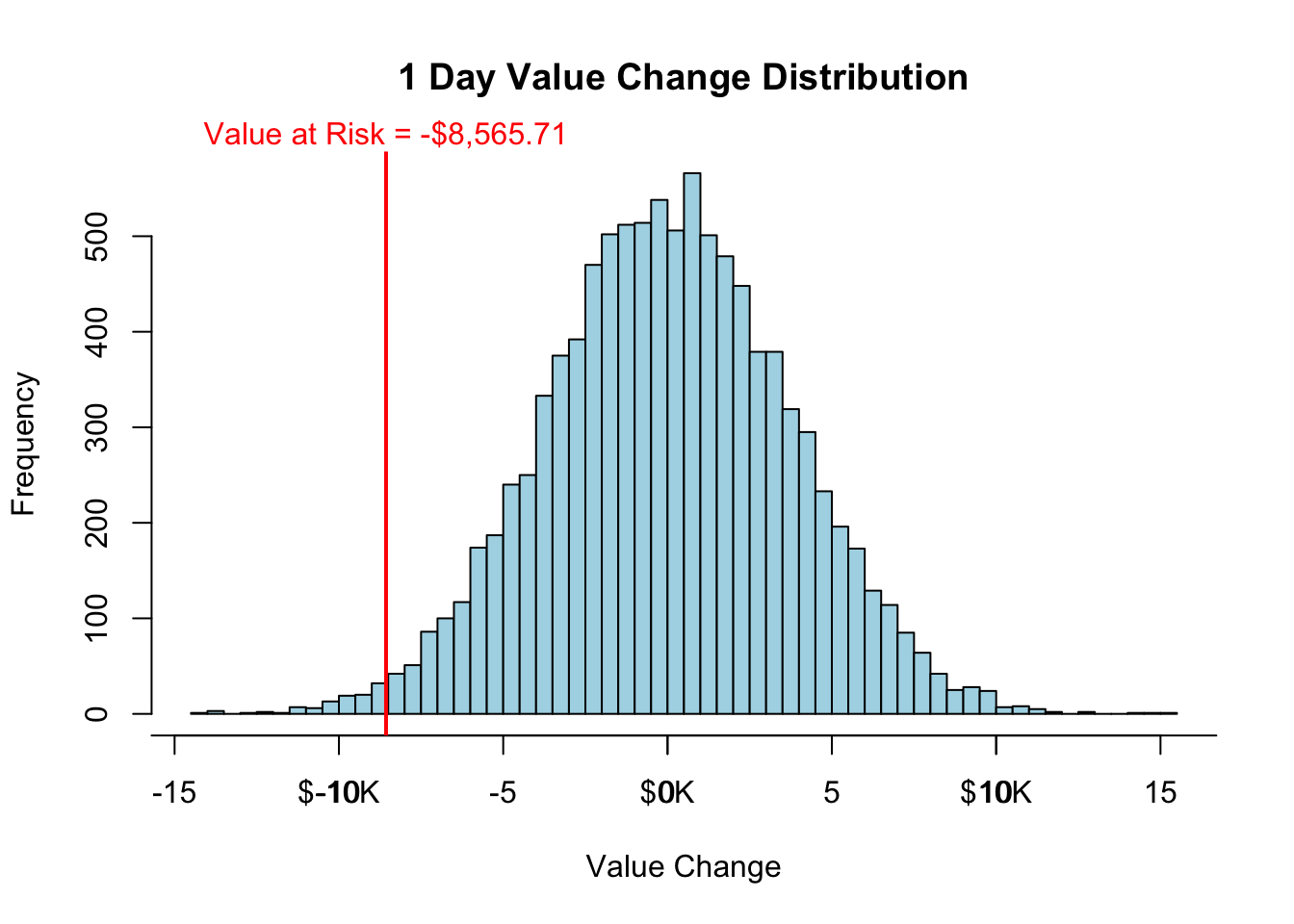
The one day, 1% VaR for this portfolio calculated above assumes normality of returns for each asset. If this is not true, then the VaR is an incorrect estimate.
Running this simulation is rather easy to do in Python. First, we define our correlation structure (here R) and calculate the Cholesky decomposition of this matrix to multiply into our data. Next, we simulate 10,000 draws from the respective normal distributions for our Microsoft and Apple returns using the rnorm function. We multiply in the correlation structure and then simply calculate the return on the portfolio of these two sets of returns. From there it is a simple call of the quantile function to find the quantile of the distribution to get the VaR. A histogram of the distribution of changes in the portfolio is also provided. For more details on how to run simulations in Python, please see the code notes for Introduction to Simulation.
import scipy as sp
import pandas as pd
import seaborn as sns
import matplotlib.pyplot as plt

n_simulations = 10000
R = np.array([[1, cor_m_a], [cor_m_a, 1]])
U = sp.linalg.cholesky(R, lower = False)

msft_r = np.random.normal(loc = np.mean(stocks['msft_r']), scale = np.sqrt(var_msft), size = n_simulations)
aapl_r = np.random.normal(loc = np.mean(stocks['aapl_r']), scale = np.sqrt(var_aapl), size = n_simulations)
Both_r = np.array([msft_r, aapl_r])
port_r = U @ Both_r
port_r = np.transpose(port_r)

port_v = MSFT_inv*port_r[:,0] + AAPL_inv*port_r[:,1]

VaR = np.quantile(port_v, VaR_percentile)
locale.currency(VaR, grouping = True)
'-$8,438.65'
value_df = pd.DataFrame(port_v)

ax = sns.histplot(data = value_df)
ax.set_title('One-Day Value Change Distribution')
ax.set_xlabel("Value Change")
ax.axvline(x = VaR, color = "red")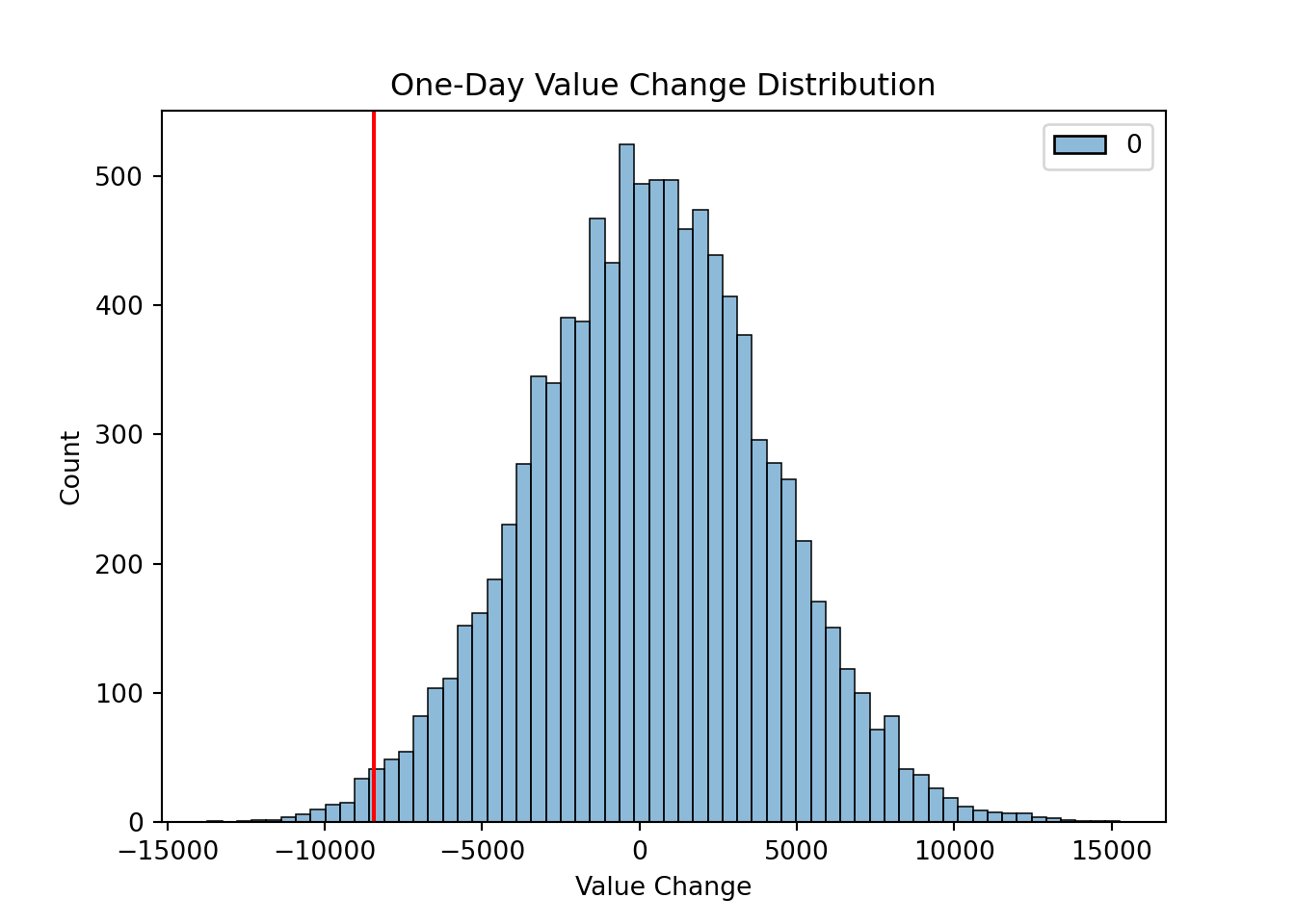
The one day, 1% VaR for this portfolio calculated above assumes normality of returns for each asset. If this is not true, then the VaR is an incorrect estimate.
Running this simulation is a little complicated in SAS due to correlation structure we are imposing on the returns. For more detail on the code below and the approach to adding in correlation structures in simulations in SAS please see the code notes for Introduction to Simulation. First, we define our correlation structure using the DATA step. This will repeat the desired correlation matrix the number of times we are simulating. Next, we again use the DATA step to define starting points for each of the variables in the simulation - namely the returns for Microsoft and Apple. From there PROC MODEL simulates and correlates the necessary returns.
data Corr_Matrix;
    do i=1 to 10000;
        _type_ = "corr";
        _name_ = "msft_r";

        msft_r = 1.0;
        aapl_r = &corr;

        output;
        _name_ = "aapl_r";

        msft_r = &corr;
        aapl_r = 1.0;

        output;
    end;
run;

data Naive;
    do i=1 to 10000;
        msft_r=0;
        aapl_r=0;
        output;
    end;
run;

proc model noprint;

    msft_r = 0;
    errormodel msft_r ~Normal(&var_msft);

    aapl_r = 0;
    errormodel aapl_r ~Normal(&var_aapl);

    solve msft_r aapl_r/ random=1 sdata=Corr_Matrix
    data=Naive out=mc_stocks(keep=msft_r aapl_r i);
        by i;

run;
quit;

data mc_stocks;
    set mc_stocks;
    by i;
    if first.i then delete;
    rename i=simulation;
    value_change = &msft_position*msft_r + &aapl_position*aapl_r;
    value = &msft_position + &aapl_position + value_change;
    format value_change dollar15.2;
run;

%let var_clevel=%sysevalf(100*&var_percentile);

proc univariate data=mc_stocks;
    var value_change;
    format value_change dollar15.2;
    output out=percentiles pctlpts = &var_clevel pctlpre=P;
    histogram value_change / kernel normal;
  ods select Quantiles;
run;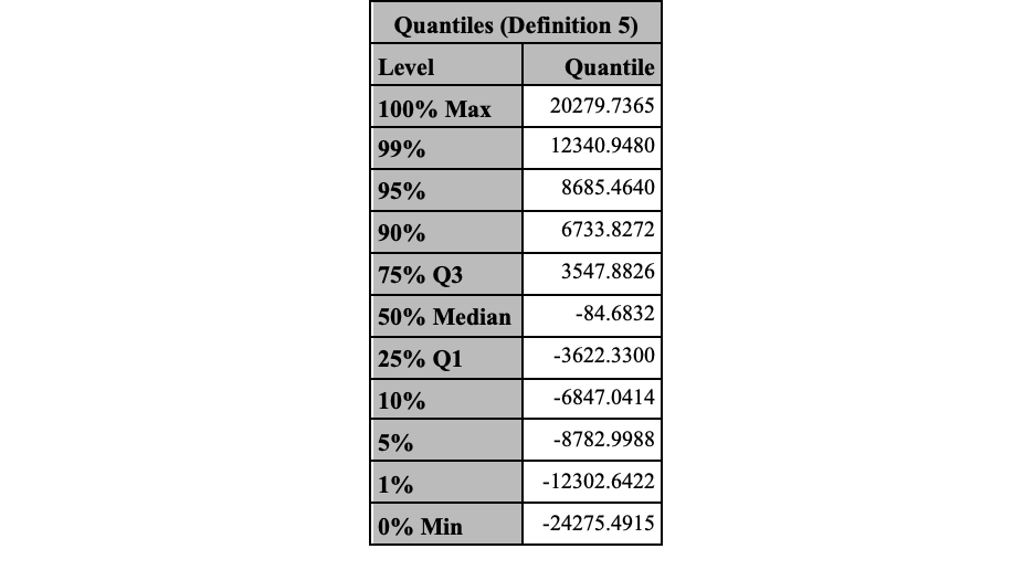
The one day, 1% VaR for this portfolio calculated above assumes normality of returns for each asset. If this is not true, then the VaR is an incorrect estimate.
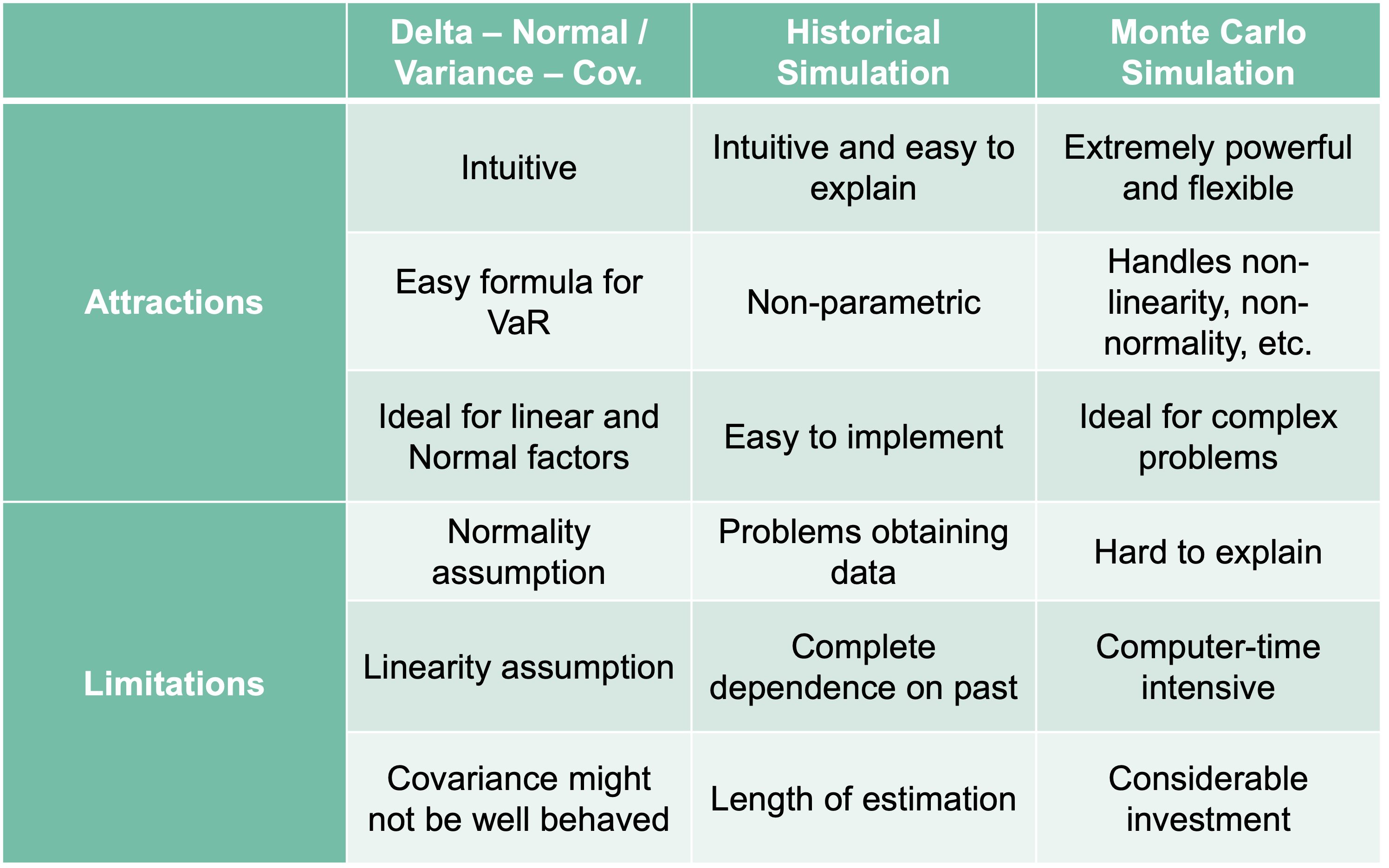
The following is a summary comparison for the three approaches - Delta-Normal, historical simulation, and simulation.
Value at risk calculations in any of the above approaches are just estimates. All estimates have a notion of variability. Therefore, we can calculate confidence intervals for each of the above approaches.
When you have a normal distribution (the Delta-Normal approach) there is a known mathematical equation for the confidence interval around a quantile. It is derived as a confidence interval around the standard deviation \(\sigma\) followed by multiplying this \(\sigma\) by the corresponding quantiles of interest on the normal distribution. The confidence interval for \(\sigma\) is as follows:
\[ CI(\hat{\sigma}) = (\sqrt{\frac{(n-1) \sigma^2}{\chi^2_{\alpha/2, n-1}}}, \sqrt{\frac{(n-1) \sigma^2}{\chi^2_{1-\alpha/2, n-1}}}) \]
For non-normal distributions or historical / simulation approaches, the bootstrap method of confidence intervals is probably best. The bootstrap approach to confidence intervals is as follows:
Resample from the simulated data using their empirical distribution; or rerun the simulation several times.
In each new sample (from step 1) calculate the VaR.
Repeat steps 1 and 2 many times to get several VaR estimates. Use these estimates to get the expected VaR and its confidence interval.
Let’s see both of these approaches in our software!
Let’s first start with the direct normal distribution calculation approach. Under the Delta-Normal approach you can easily calculate the confidence interval for the value at risk based on the equation defined above. The code below just recreates that function using the qchisq and qnorm functions were necessary to get values from the \(\chi^2\) and normal distributions.
sigma.low <- sqrt(var.port*(length(stocks$AAPL.Close)-1)/qchisq((1-(VaR.percentile/2)),length(stocks$AAPL.Close)-1) )Warning in qchisq((1 - (VaR.percentile/2)), length(stocks$AAPL.Close) - : NaNs
producedsigma.up <- sqrt(var.port*(length(stocks$AAPL.Close)-1)/qchisq((VaR.percentile/2),length(stocks$AAPL.Close)-1) )Warning in qchisq((VaR.percentile/2), length(stocks$AAPL.Close) - 1): NaNs
producedVaR.DN.port <- (AAPL.inv+MSFT.inv)*qnorm(VaR.percentile)*sqrt(var.port)
VaR.L <- (AAPL.inv+MSFT.inv)*qnorm(VaR.percentile)*(sigma.low)
VaR.U <- (AAPL.inv+MSFT.inv)*qnorm(VaR.percentile)*(sigma.up)
print(paste("The VaR is ", dollar(VaR.DN.port), " with confidence interval (", dollar(VaR.L), " , ", dollar(VaR.U), ")", sep = "" ))[1] "The VaR is -$8,530.90 with confidence interval (NA , NA)"To perform the bootstrap approach in R, we first need to define the number of bootstrap samples as well as the size of each of these samples. From there we loop through the simulation values we already obtained earlier called value.change using a for loop. Using the sample function we can sample values from our original simulation and calculate the VaR of this new sub-sample using the quantile function at our percentile. We repeat this process over and over until we form many different values for our VaR from which to build our confidence interval. From there we simply look at the values that define the middle 95% of all of our VaR values, again using the quantile function to define the upper and lower bounds of our confidence interval. Lastly, we plot the VaR as well as its confidence interval bounds on a histogram of the value.change distribution.
n.bootstraps <- 1000
sample.size <- 1000

VaR.boot <- rep(0,n.bootstraps)
for(i in 1:n.bootstraps){
  bootstrap.sample <- sample(value.change, size=sample.size)
  VaR.boot[i] <- quantile(bootstrap.sample, VaR.percentile, na.rm=TRUE)
}

VaR.boot.U <- quantile(VaR.boot, 0.975, na.rm=TRUE)
VaR.boot.L <- quantile(VaR.boot, 0.025, na.rm=TRUE)

print(paste("The VaR is ", dollar(mean(VaR.boot)), " with confidence interval (", dollar(VaR.boot.L), " , ", dollar(VaR.boot.U), ")", sep = "" ))
[1] "The VaR is -$8,464.71 with confidence interval (-$9,400.30 , -$7,668.54)"hist(value.change/1000, breaks=50, main='1 Day Value Change Distribution', xlab='Value Change', col="lightblue")
breaks = c(-20, -10, 0, 10, 20)
axis(1, at = breaks, labels = paste("$", breaks, "K", sep = ""))
abline(v = VaR/1000, col="red", lwd=2)
mtext(paste("Value at Risk",VaR.label, sep=" = "), at = VaR/1000, col="red")
abline(v = VaR.boot.L/1000, col="blue", lwd=2, lty="dashed")
abline(v = VaR.boot.U/1000, col="blue", lwd=2, lty="dashed")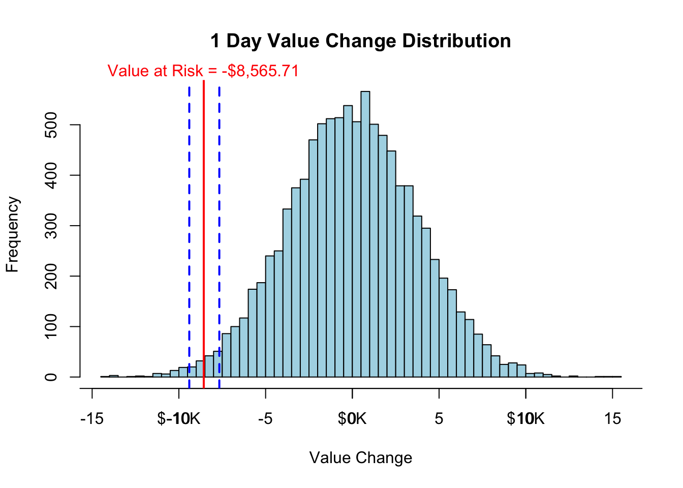
Let’s first start with the direct normal distribution calculation approach. Under the Delta-Normal approach you can easily calculate the confidence interval for the value at risk based on the equation defined above. The code below just recreates that function using the chi2.ppf and norm.ppf functions from numpy were necessary to get values from the \(\chi^2\) and normal distributions.
sigma_low = np.sqrt(var_port * (stocks.shape[0] - 1) / sps.chi2.ppf((1 - VaR_percentile/2), (stocks.shape[0] - 1)))
sigma_up = np.sqrt(var_port * (stocks.shape[0] - 1) / sps.chi2.ppf((VaR_percentile/2), (stocks.shape[0] - 1)))

VaR_DN_port = (AAPL_inv+MSFT_inv)*sps.norm.ppf(VaR_percentile)*np.sqrt(var_port)
VaR_L = (AAPL_inv+MSFT_inv)*sps.norm.ppf(VaR_percentile)*sigma_low
VaR_U = (AAPL_inv+MSFT_inv)*sps.norm.ppf(VaR_percentile)*sigma_up

print("The VaR is", locale.currency(VaR_DN_port, grouping = True), "with confidence interval (", locale.currency(VaR_L, grouping = True), ",", locale.currency(VaR_U, grouping = True), ")" )
The VaR is -$8,542.70 with confidence interval ( -$7,895.73 , -$9,296.21 )To perform the bootstrap approach in Python, we first need to define the number of bootstrap samples as well as the size of each of these samples. From there we loop through the simulation values we already obtained earlier called value_df using a for loop. Using the sample function we can sample values from our original simulation and calculate the VaR of this new sub-sample using the quantile function at our percentile. We repeat this process over and over until we form many different values for our VaR from which to build our confidence interval. From there we simply look at the values that define the middle 95% of all of our VaR values, again using the quantile function from numpy to define the upper and lower bounds of our confidence interval. Lastly, we plot the VaR as well as its confidence interval bounds on a histogram of the value_df distribution.
n_bootstraps = 1000
sample_size = 1000

data = []
for i in range(n_bootstraps):
  bootstrap_sample = value_df.sample(n = sample_size)
  VaR_boot = np.quantile(bootstrap_sample, VaR_percentile)
  data.append(VaR_boot)

VaR_boot_U = np.quantile(data, 0.975)
VaR_boot_L = np.quantile(data, 0.025)

print("The VaR is", locale.currency(np.mean(data), grouping = True), "with confidence interval (", locale.currency(VaR_boot_L, grouping = True), ",", locale.currency(VaR_boot_U, grouping = True), ")" )
The VaR is -$8,384.52 with confidence interval ( -$9,012.84 , -$7,715.03 )
ax = sns.histplot(data = value_df)
ax.set_title('One-Day Value Change Distribution')
ax.set_xlabel("Value Change")
ax.axvline(x = np.mean(data), color = "red")
ax.axvline(x = VaR_boot_L, color = "blue", ls = "--")
ax.axvline(x = VaR_boot_U, color = "blue", ls = "--")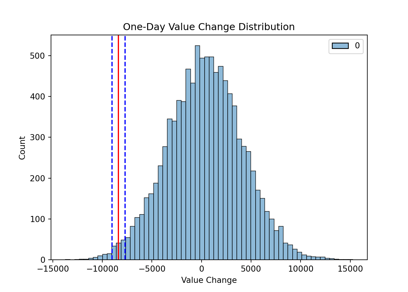
It is actually rather easy to calculate the confidence intervals for a percentile in SAS under the normality assumption. PROC UNIVARIATE and the cipctlnormal option calculates confidence intervals for percentiles of any variable. Here we define the value_change variable from our data set to make this calculation.
proc univariate data=mc_stocks cipctlnormal;
    var value_change;
  ods select Quantiles;
run;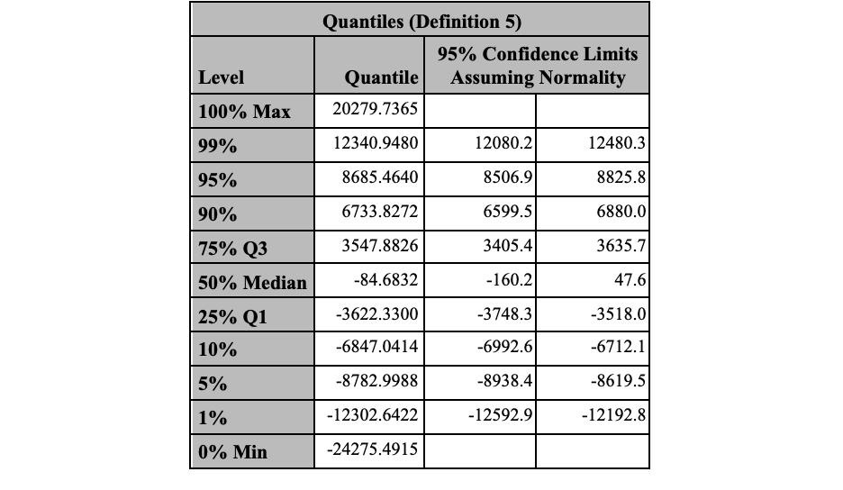
To perform the bootstrap approach in SAS, we first need to define the number of bootstrap samples as well as the size of each of these samples. From there we use PROC SURVEYSELECT to sample from our data set many times. The method = srs option specifies that we want to use simple random sampling. We want sample sizes that are 10% of the size of the simulation which is defined in the samprate = option. Lastly, we repeat this sampling over and over again using the rep = option. Make sure to put noprint so you don’t see results from each of these 1,000 samples!
Next, we just calculate percentiles using PROC UNIVARIATE for each of the samples (called replicates) using the by statement. We will output the percentiles from each of these calculations using the output statement with the out = option. Specifically, we want the 1% quantile (our VaR values) which we can define using the pctlpts option. We will label this quantile as P1. We define this name using the pctlpre option to define the prefix on the number of the quantile (here 1). Another PROC UNIVARIATE call will give us the percentiles of all of these VaR calculations from the previous PROC UNIVARIATE. Lastly, we print these results.
%let n_bootstraps=1000;
%let bootstrap_prop=0.1;
%let var_percentile = 0.01;
%let var_clevel=%sysevalf(100*&var_percentile);

proc surveyselect data=mc_stocks out=outboot seed=12345 method=srs
                  samprate=&bootstrap_prop rep=&n_bootstraps noprint;
run;

proc univariate data=outboot noprint;
    var value_change;
    output out=boot_var pctlpts = &var_clevel pctlpre=P;
    by replicate;
run;

proc univariate data=boot_var;
    var P1;
    output out=var_ci pctlpts = 2.5 97.5 pctlpre=P;
  ods select Quantiles;
run;

proc print data=var_ci;
run;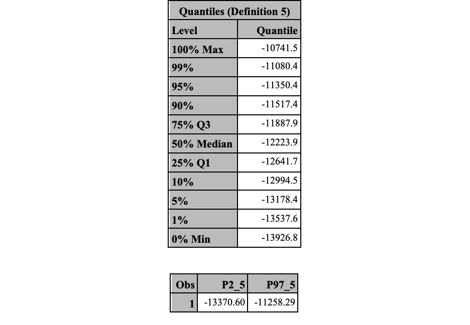
The ES is a conditional expectation that tries to answer what you should expect to lose if your loss exceeds the VaR. It is the expected (average) value of the portfolio in the circled region below:
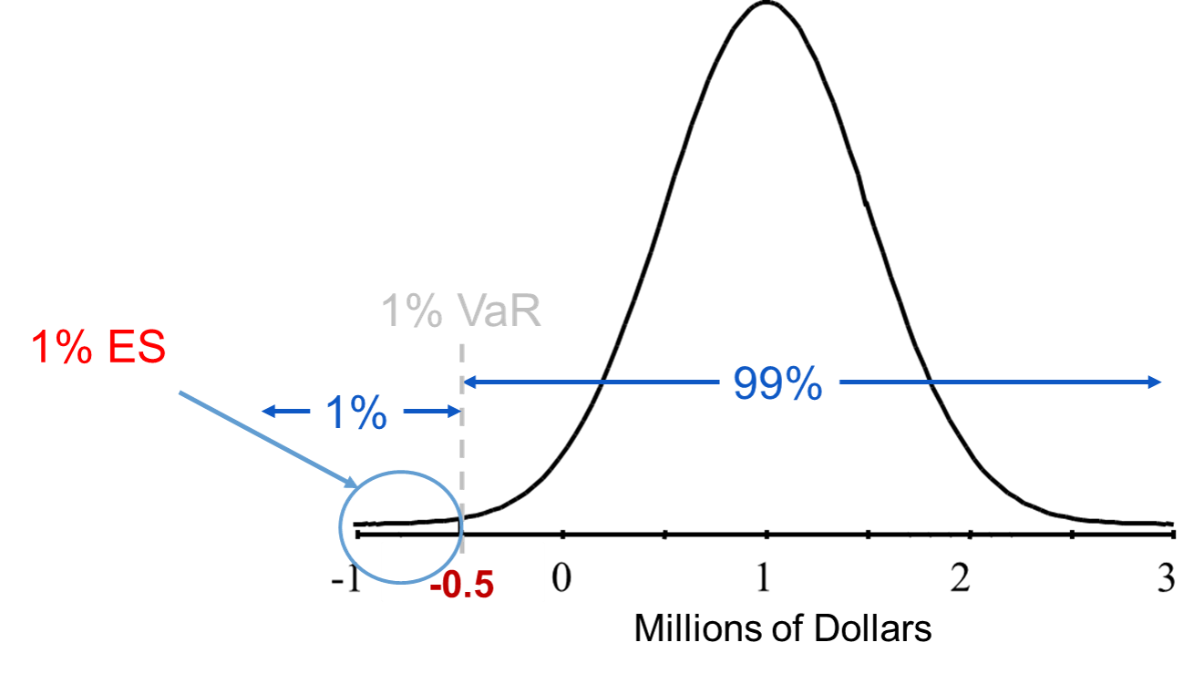
The main question is how to estimate the distribution that we will calculate the average of the worst case outcomes. There are three main approaches to estimating the distribution in ES and they are the same as VaR:
Delta-Normal (Variance-Covariance) Approach
Historical Simulation Approach(es)
Simulation Approach
The best part is that extending these approaches to include expected shortfall from what we already covered for value at risk is rather straight forward. Let’s take a look at each of these.
Just like the VaR calculation for the Delta-Normal approach, the ES has a known equation. For a normal distribution, the average (or expected value) in a tail of the distribution is defined as follows:
\[ ES = CVaR = \mu - \sigma \times \frac{e^{-q^2_{\alpha/2}}}{\alpha \sqrt{2 \pi}} \]
with \(\sigma\) being the standard deviation of the data, \(\alpha\) being the percentile of interest (1% for example), and \(q_{\alpha}\) as the tail percentile from the standard normal distribution (-2.33 for example).
Let’s see how to code this into our software!
Just as with the VaR, the ES is easy to hard code into R directly. The function below repeats the same function as defined above.
ES.DN.port <- (0 - sqrt(var.port)*exp(-(qnorm(VaR.percentile)^2)/2)/(VaR.percentile*sqrt(2*pi)))*(AAPL.inv+MSFT.inv)
dollar(ES.DN.port)
[1] "-$9,773.55"Just as with the VaR, the ES is easy to hard code into Python directly. The function below repeats the same function as defined above.
ES_DN_port = (0 - np.sqrt(var_port) * np.exp(-(sps.norm.ppf(VaR_percentile)**2)/2)/(VaR_percentile * np.sqrt(2 * np.pi)))*(AAPL_inv + MSFT_inv)

locale.currency(ES_DN_port, grouping = True)'-$9,787.06'Just as with the VaR, the ES can be coded into SAS directly using PROC IML. The function below repeats the same function as defined above.
%let msft_position = 200000;
%let aapl_position = 100000;
%let var_percentile = 0.01;

proc iml;
title 'VaR Results';

msft_p_weight = &msft_position/(&msft_position + &aapl_position);
aapl_p_weight = &aapl_position/(&msft_position + &aapl_position);

P_variance =  &var_msft*(msft_p_weight)**2 + &var_aapl*(aapl_p_weight)**2
                   + 2*aapl_p_weight*msft_p_weight*&covar;
P_StdDev=sqrt(P_variance);

VaR_normal = (&msft_position + &aapl_position)*PROBIT(&var_percentile)*SQRT(P_variance);

pi=3.14159265;
ES_normal = -(&msft_position + &aapl_position)*SQRT(P_variance)*exp(-0.5*(PROBIT(&var_percentile))**2)/(&var_percentile.*sqrt(2*pi));

print "Daily CVaR/ES (Percentile level: &var_percentile); Delta-Normal" ES_normal[format=dollar15.2];

quit;
The calculation above would be the average of the 1% worst case scenarios, assuming normality was true.
We can easily extend the historical simulation approach for VaR to ES. Let’s look at our two position portfolio example. Suppose you invested $200,000 in Microsoft and $100,000 in Apple today. You have 500 historical observations on both returns. Simply calculate the portfolio’s value as if each of the previous 500 days is a possible scenario for your one day return on this portfolio. We then sort these 500 possible scenarios and the 1% ES will be the average of these 5 observations that make up the 1%:
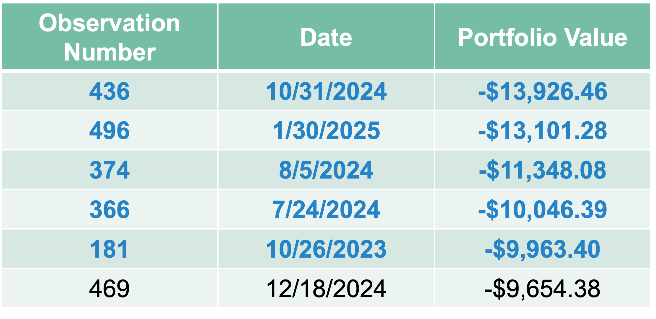
The average of these 5 observations is -$11,677.12. Again, this value is saying that if the worst 1% of cases happens, we expect to lose $11,677.12 on average.
Let’s see how to do this in each of our software!
Just as with the historical simulation approach before for VaR, we can easily isolate the worst five observations using the head and order functions followed by using the mean to take the average.
ES.H.port <- mean(stocks$port_v[head(order(stocks$port_v), 5)])
dollar(as.numeric(ES.H.port))
[1] "-$11,952.69"Just as with the historical simulation approach before for VaR, we can easily isolate the worst five observations using the head and sort_values functions followed by using the mean to take the average.
ES_H_port = np.mean(stocks['port_v'].sort_values().head(5))

locale.currency(ES_H_port, grouping = True)'-$11,677.12'Just as with the historical simulation approach before for VaR, we can easily isolate the worst five observations using PROC IML. Inside of this PROC we can calculate the mean of the worst five observations.
proc iml;

use SimRisk.stocks var {msft_r aapl_r};
read all var _all_ into returns;

portfolio_return = &msft_position*returns[,1] + &aapl_position*returns[,2];

call sort(portfolio_return,{1});
number_of_observations = nrow(portfolio_return);

VaR_historical = portfolio_return[6,1];

ES = sum(portfolio_return[1:6,1])/(6-1);
print "Daily CVaR/ES (Percentile level: &var_percentile level); Historical" ES[format=dollar15.2];


title;
quit;
The calculation above would be the average of the 1% worst case scenarios, according to historical data.
Simulation is just an extension of what we did earlier to calculate the VaR. First, follow the steps described earlier to create the 10,000 simulated, sorted, portfolio values for the VaR calculation. Then simply just take the average of all the values that are worst than the VaR. For 10,000 simulations, the ES would be the average of the worst 100 observations.
Let’s see how to do this in each of our software!
Just as with simulation in R, we can easily get the final distribution for our portfolio changes, called value.change, and just isolate the worst observations through Boolean logic. We just take the mean function of all the observations for value.change that are lower than the VaR value.
ES <- mean(value.change[value.change < VaR], na.rm=TRUE)
dollar(ES)
[1] "-$9,864.40"h <- hist(value.change/1000, breaks=50, plot=FALSE)
cuts <- cut(h$breaks, c(-Inf, VaR/1000, Inf))
plot(h, col = cuts, main='1 Day Value Change Distribution', xlab='Value Change')
breaks = c(-20, -10, 0, 10, 20, 30)
axis(1, at = breaks, labels = paste("$", breaks, "K", sep = ""))
abline(v = VaR/1000, col="red", lwd=2)
mtext(paste("Value at Risk",VaR.label, sep=" = "), at=VaR/1000, col="red")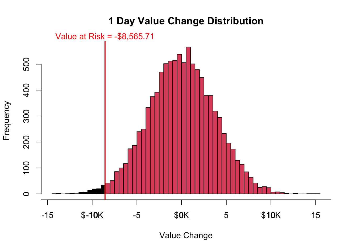
Just as with simulation in Python, we can easily get the final distribution for our portfolio changes, called port_v, and just isolate the worst observations through Boolean logic. We just take the mean function of all the observations for port_v that are lower than the VaR value.
ES = np.mean(port_v[port_v < VaR])

locale.currency(ES, grouping = True)'-$9,538.77'Just as with simulation in SAS, we can easily get the final distribution for our portfolio changes, called value_change in our mc_stocks data set, and just isolate the worst observations through the WHERE statement in PROC MEANS. This will apply the mean of all the observations for value_change that are lower than the VaR value.
proc print data=percentiles;
run;

data _null_;
    set percentiles;
    call symput("var_p",P1);
run;

proc means data=mc_stocks mean;
    var value_change;
    where value_change < &var_p;
run;
Again, the above value is the average of the 1% worst case scenarios, assuming our structure of the simulations is correct.