
Binary Logistic Regression
Introduction
These notes will primarily focus on binary logistic regression. It is the most common type of logistic regression, and sets up the foundation for more complicated versions - ordinal and nominal logistic regression.
Regression is modeling the expected (mean/average) of the target variable conditional on the predictors:
\[ E(y_i | x_{1,i}, x_{2,i}, \ldots) \]
For a binary (0/1) target variable, \(y_i\), the expected value is just the probability of the event:
\[ E(y_i) = P(y_1 = 1) = p_i \]
This could lead us to thinking that we should model the following:
\[ p_i = \beta_0 + \beta_1 x_{1,i} + \cdots + \beta_k x_{k,i} \]
That is called the linear probability model. This is not the best model to use to model probabilities as logistic regression models are more designed for modeling probabilities. However, for completeness sake however, let’s discuss the linear probability model.
Linear Probability Model
The linear probability model is not as widely used since probabilities do not tend to follow the properties of linearity in relation to their predictors. Also, the linear probability model possibly produces predictions outside of the bounds of 0 and 1 (where probabilities should be!).
Let’s first view what a linear probability model would look like plotted on our data and then we can build the model.
Even though it doesn’t appear to really look like our data, let’s fit this linear probability model anyway for completeness sake. Only the results are shown below.
| Dep. Variable: | bonus | R-squared: | 0.312 |
| Model: | OLS | Adj. R-squared: | 0.312 |
| Method: | Least Squares | F-statistic: | 496.4 |
| Date: | Sat, 15 Nov 2025 | Prob (F-statistic): | 5.88e-91 |
| Time: | 10:54:40 | Log-Likelihood: | -579.24 |
| No. Observations: | 1095 | AIC: | 1162. |
| Df Residuals: | 1093 | BIC: | 1172. |
| Df Model: | 1 | ||
| Covariance Type: | nonrobust |
| coef | std err | t | P>|t| | [0.025 | 0.975] | |
| Intercept | -0.3581 | 0.038 | -9.540 | 0.000 | -0.432 | -0.284 |
| GrLivArea | 0.0005 | 2.32e-05 | 22.280 | 0.000 | 0.000 | 0.001 |
| Omnibus: | 1.803 | Durbin-Watson: | 2.173 |
| Prob(Omnibus): | 0.406 | Jarque-Bera (JB): | 1.759 |
| Skew: | -0.032 | Prob(JB): | 0.415 |
| Kurtosis: | 3.186 | Cond. No. | 4.88e+03 |
Notes:
[1] Standard Errors assume that the covariance matrix of the errors is correctly specified.
[2] The condition number is large, 4.88e+03. This might indicate that there are
strong multicollinearity or other numerical problems.
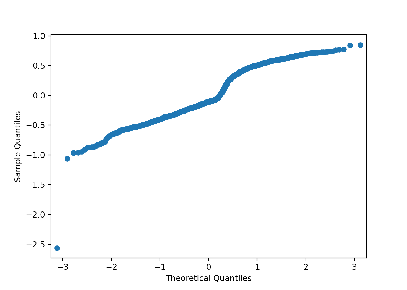
As we can see from the charts above, the assumptions of ordinary least squares don’t really hold in this situation. Therefore, we should be careful interpreting the results of the model. Maybe a better model won’t have these problems?
Binary Logistic Regression Model
Due to the limitations of the linear probability model, people typically just use the binary logistic regression model. The logistic regression model does not have the limitations of the linear probability model. The outcome of the logistic regression model is the probability of getting a 1 in a binary variable, \(E(y_i) = P(y_i = 1) = p_i\). That probability is calculated as follows:
\[ p_i = \frac{1}{1+e^{-(\beta_0 + \beta_1x_{1,i} + \cdots + \beta_k x_{k,i})}} \]
This function has the desired properties for predicting probabilities. The predicted probability from the above equation will always be between 0 and 1. The parameter estimates do not enter the function linearly (this is a non-linear regression model), and the rate of change of the probability varies as the predictor variables vary as seen below.
(-0.05, 1.05)
To create a linear model, a link function is applied to the probabilities. The specific link function for logistic regression is called the logit function.
\[ logit(p_i) = \log(\frac{p_i}{1-p_i}) = \beta_0 + \beta_1x_{1,i} + \cdots + \beta_k x_{k,i} \]
The relationship between the predictor variables and the logits are linear in nature as the logits themselves are unbounded. This structure looks much more like our linear regression model structure. However, logistic regression does not use ordinary least squares (OLS) to estimate the coefficients in our model. OLS requires residuals which the logistic regression model does not provide. The target variable is binary in nature, but the predictions are probabilities. Therefore, we cannot calculate a traditional residual. The estimation method for logistic regression is discussed after we build our first model.
Let’s see how to run binary logistic regression in each software!
The Logit function and the fit attribute in Python from the statsmodels.api package will provide us the ability to model binary logistic regressions. With this function you can specify a model using the usual X and y objects. We will use a smaller dataset that we will call X_little. This dataset will include only two variables - GrLivArea and CentralAir_Y. The summary function provides the output from this model.
Code
import statsmodels.api as sm

# Create Small Dataset for Example
X_little = X[['GrLivArea','CentralAir_Y']]
X_little = sm.add_constant(X_little)

# Build Logistic Regression
model = sm.Logit(y, X_little)
result = model.fit()
Optimization terminated successfully.
Current function value: 0.442355
Iterations 8Code
print(result.summary()) Logit Regression Results
==============================================================================
Dep. Variable: bonus No. Observations: 1095
Model: Logit Df Residuals: 1092
Method: MLE Df Model: 2
Date: Sat, 15 Nov 2025 Pseudo R-squ.: 0.3529
Time: 10:54:41 Log-Likelihood: -484.38
converged: True LL-Null: -748.55
Covariance Type: nonrobust LLR p-value: 1.868e-115
================================================================================
coef std err z P>|z| [0.025 0.975]
--------------------------------------------------------------------------------
const -11.3561 1.012 -11.222 0.000 -13.339 -9.373
GrLivArea 0.0042 0.000 15.531 0.000 0.004 0.005
CentralAir_Y 4.8704 0.836 5.825 0.000 3.232 6.509
================================================================================Let’s examine the output above. Scanning down the output, you can see the actual logistic regression equation itself for each of the variables. At our significance level (we used an 0.009 significance level for this analysis based on the sample size) it appears that both of these variables are significant.
The glm function in R will provide us the ability to model binary logistic regressions. Similar to the lm function, you can specify a model formula. Notice the factor function on the CentralAir variable. This will convert this categorical variable into usable design variables for the modeling function.
The family = binomial(link = "logit") option is there to specify that we are building a logistic model. Generalized linear models (GLM) are a general class of models where logistic regression is a special case where the link function is the logit function. Use the summary function to look at the necessary output.
Code
logit.model <- glm(bonus ~ GrLivArea + factor(CentralAir),
data = train, family = binomial(link = "logit"))
summary(logit.model)
Call:
glm(formula = bonus ~ GrLivArea + factor(CentralAir), family = binomial(link = "logit"),
data = train)
Coefficients:
Estimate Std. Error z value Pr(>|z|)
(Intercept) -11.356071 1.011793 -11.224 < 2e-16 ***
GrLivArea 0.004163 0.000268 15.531 < 2e-16 ***
factor(CentralAir)Y 4.870388 0.835919 5.826 5.66e-09 ***
---
Signif. codes: 0 '***' 0.001 '**' 0.01 '*' 0.05 '.' 0.1 ' ' 1
(Dispersion parameter for binomial family taken to be 1)
Null deviance: 1497.10 on 1094 degrees of freedom
Residual deviance: 968.76 on 1092 degrees of freedom
AIC: 974.76
Number of Fisher Scoring iterations: 6Let’s examine the output above. Scanning down the output, you can see the actual logistic regression equation itself for each of the variables, including the design variable created for CentralAir with the factor function. At our significance level (we used an 0.009 significance level for this analysis based on the sample size) it appears that both of these variables are significant.
Coefficient Interpretations
One of the benefits of logistic regression is the interpretability of the model. The coefficients from the logistic regression model are interpretable, just not in the exact sense of linear regression. The coefficients in the logistic regression are the foundation of calculating odds ratios.
An odds ratio indicates how much more likely, with respect to odds, a certain event occurs in one group relative to its occurrence in another group. The odds of an event occurring is not the same as the probabilities that an event occurs, but related to the probability an event occurs:
\[ Odds = \frac{p}{1-p} \]
Notice how those odds form the foundation of the logit equation from before:
\[ logit(p_i) = \log(\frac{p_i}{1-p_i}) = \beta_0 + \beta_1x_{1,i} + \cdots + \beta_k x_{k,i} \]
The logit is the natural log of the odds of an event occurring. That means we could take the exponential of the logit function output and get the odds. However, if we were to take the ratio of two of these we would get the interpretable odds ratio. For example, let’s look at comparing the odds of a home with central air conditioning and without. We use the output from the logistic regression above to get the following equations:
\[ Odds_Y = e^{-11.36 + 4.87*CentralAir_Y + 0.0042*GrLivArea} = e^{-11.36 + 4.87(1) + 0.0042*GrLivArea} \]
\[ Odds_N = e^{-11.36 + 4.87*CentralAir_Y + 0.0042*GrLivArea} = e^{-11.36 + 4.87(0) + 0.0042*GrLivArea} \]
Let’s now take the ratio of those equations:
\[ OR = \frac{e^{-11.36 + 4.87(1) + 0.0042*GrLivArea}}{e^{-11.36 + 4.87(0) + 0.0042*GrLivArea}} \]
The intercept term as well as the GrLivArea variable all cancel themselves out leaving only the exponential function of the original coefficient on the CentralAir_Y variable:
\[ OR = \frac{e^{-11.36 + 4.87(1) + 0.0042*GrLivArea}}{e^{-11.36 + 4.87(0) + 0.0042*GrLivArea}} = \frac{e^{-11.36} e^{4.87(1)} e^{0.0042*GrLivArea}}{e^{-11.36} e^{0} e^{0.0042*GrLivArea}} = e^{4.87} = 130.37 \]
This gives the odds ratio. The interpretation on this ratio is that homes with central air are 130.37 times as likely to be bonus eligible than homes without central air, on average.
The same math can be done if we wanted to interpret the increase of a continuous variable by 1 unit. Let’s interpret the impact on odds of bonus eligibility when we increase the square footage by 1:
\[ OR = \frac{e^{-11.36 + 4.87*CentralAir_Y + 0.0042*(GrLivArea + 1)}}{e^{-11.36 + 4.87*CentralAir_Y + 0.0042*GrLivArea}} \]
\[ OR = \frac{e^{-11.36} e^{4.87*CentralAir_Y} e^{0.0042*GrLivArea} e^{0.0042}}{e^{-11.36} e^{4.87*CentralAir_Y} e^{0.0042*GrLivArea}} = e^{0.0042} = 1.0042 \]
The interpretation on this ratio is that every extra square footage on the home makes the odds of bonus eligibility 1.0042 times as likely to occur, on average. Due to the small scale of this increase, it makes it harder to interpret. Instead we could perform the following transformation:
\[ 100\times (OR -1)\% \]
Now our interpretation would be that every additional square foot of space expects to have 0.42% (= \(100 \times (e^{0.0042} - 1)\) ) higher odds to be bonus eligible. If this resulted in a negative number, it would be lower odds of bonus eligibility.
Just for fun, we can work through the math backwards to see what increase in square footage is needed for an expected doubling of the odds of a home being bonus eligible. The estimated amount to double the odds is the following:
\[ Double Odds = \frac{\log(2)}{\beta} = \frac{\log(2)}{0.0042} = 165.02 \]
Therefore, every additional increase of 165 square feet to the home doubles the odds of bonus eligibility, on average.
Let’s see how to calculate this in each software!
Odds ratios are not hard to calculate once we obtain the coefficients from our model. The params function provides the coefficients once applied to the model object, here result.
Code
import numpy as np
OR = np.exp(result.params)
print(OR)const 0.000012
GrLivArea 1.004171
CentralAir_Y 130.371569
dtype: float64Odds ratios are a great way of interpreting the output from a logistic regression. For example, let’s look at the CentralAir_Y variable odds ratio. This tells us that homes with central air are 130.7 times as likely (in terms of odds) of being bonus eligible, on average, then homes without central air. To practice interpreting continuous variables, let’s look at the GrLivArea variable. Every additional square foot of living area leads to the home being 1.0042 times as likely to be bonus eligible. This maybe a little harder to easily understand. Another way to put this would be that every additional square foot of living area increases the odds of the home being bonus eligible by 0.42% (100*(1.0042 - 1)) on average.
Code
OR = 100*(np.exp(result.params) - 1)
print(OR)const -99.998830
GrLivArea 0.417133
CentralAir_Y 12937.156941
dtype: float64Odds ratios are not hard to calculate once we obtain the coefficients from our model. The coef function provides the coefficients once applied to the model object, here logit.model. We can also get confidence intervals around the coefficients using the confint function.
Code
exp(
cbind(coef(logit.model), confint(logit.model))
) 2.5 % 97.5 %
(Intercept) 1.169825e-05 1.250669e-06 7.212233e-05
GrLivArea 1.004171e+00 1.003662e+00 1.004718e+00
factor(CentralAir)Y 1.303716e+02 3.069894e+01 9.287957e+02Odds ratios are a great way of interpreting the output from a logistic regression. For example, let’s look at the CentralAir variable odds ratio. This tells us that homes with central air are 130.37 times as likely (in terms of odds) of being bonus eligible, on average, then homes without central air. To practice interpreting continuous variables, let’s look at the GrLivArea variable. Every additional square foot of living area leads to the home being 1.0042 times as likely to be bonus eligible. This maybe a little harder to easily understand. Another way to put this would be that every additional square foot of living area increases the odds of the home being bonus eligible by 0.42% (100*(1.0042 - 1)) on average.
Estimation Method
As mentioned above, ordinary least squares is not a valid estimation method for logistic regression. Instead, logistic regression uses maximum likelihood estimation. Maximum likelihood estimation (MLE) is a very popular technique for estimating statistical models. It uses the assumed distribution (here logistic) to find the “most likely” values of the parameters to produce the data we see. In fact, it can be shown mathematically that the OLS solution in linear regression is the same as the MLE for linear regression. The likelihood function measures how probable a specific grid of \(\beta\) values is to have produced your data, so we want to maximize that function
The maximum likelihood function is based on the probability density function. For a binomial target variable, here is the likelihood function:
\[ L(\beta 's | y, x_1, x_2, \ldots ) = \prod_{i=1}^n p_i^{y_i} (1 - p_i)^{1-y_i} \]
The first piece of the likelihood function, \(p_i^{y_i}\), is the 1’s in our target variable and their respective probabilities. The second half of the function, \((1 - p_i)^{1 - y_i}\), is the 0’s in our target variable and their respective probabilities. If we use logistic regression in this likelihood function, the probabilities, \(p_i\) in the above equation, are represented with the logistic regression equation:
\[ p_i = \frac{1}{1+e^{-(\beta_0 + \beta_1x_{1,i} + \cdots + \beta_k x_{k,i})}} \]
Instead of the likelihood function, a lot of times people will estimate the natural log of the likelihood function to help make the computation easier:
\[ \log(L) = \sum_{i=1}^n{[y_i \log(p_i) + (1-y_i)\log(1-p_i)]} \]
A visual representation of maximizing this function is shown in the contour plot below. We try to find the maximum value of the likelihood function across a grid of possible \(\beta\) values.
<matplotlib.colorbar.Colorbar object at 0x32e545160>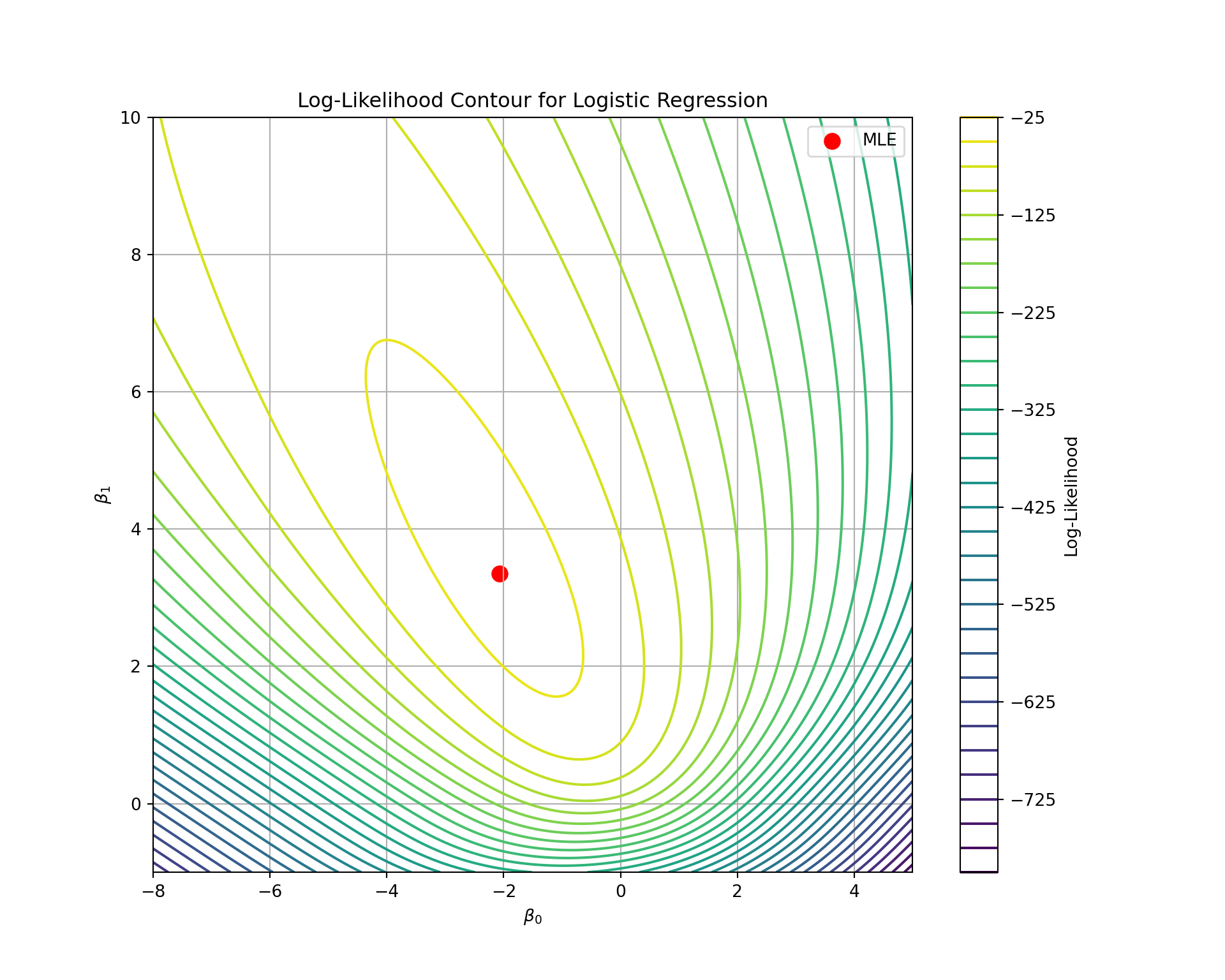
The \(\beta\) values that maximize the likelihood function are the ones that most likely produced our data and will form our estimated logistic regression model.
Likelihood Ratio Tests
Likelihood estimation provides a basis for hypothesis testing in logistic regression. If extra predictors don’t add much value / information, then a model that includes them shouldn’t be substantially more likely than the model that doesn’t include them. The likelihood ratio test (LRT) compares these full models to these reduced models. A full model is the bigger of the two models you are comparing. A reduced model is the smaller, but nested, model you are comparing. A nested model is a special case of another model. In other words, a nested model has only some of the variables that the bigger model has, but no variables that the bigger model doesn’t have. The full model will always have the same variables of the nested model plus some additional variables - the ones we are testing.
To mathematically compare these two models we compare the differences in their maximized log likelihood values. The following test statistic is based off that difference:
\[ LRT = 2 \times (\log(L_F) - \log(L_R)) \]
This test statistic follows a \(\chi^2\) distribution.
Let’s see this in each software!
Let’s build a reduced model to test the usefulness of the CentralAir_Y variable. We will still use the Logit function from the statsmodels.api package, just on the dataset without the CentralAir_Y variable. We can access the log likelihood values from each model using the llf function. From there we just calculate the test statistic as above and use the stats.chi2.sf function from scipy to get the p-value.
Code
model_red = sm.Logit(y, X_little.drop('CentralAir_Y', axis = 1))
result_red = model_red.fit()Optimization terminated successfully.
Current function value: 0.475488
Iterations 7Code
print(result_red.summary()) Logit Regression Results
==============================================================================
Dep. Variable: bonus No. Observations: 1095
Model: Logit Df Residuals: 1093
Method: MLE Df Model: 1
Date: Sat, 15 Nov 2025 Pseudo R-squ.: 0.3044
Time: 10:54:42 Log-Likelihood: -520.66
converged: True LL-Null: -748.55
Covariance Type: nonrobust LLR p-value: 3.975e-101
==============================================================================
coef std err z P>|z| [0.025 0.975]
------------------------------------------------------------------------------
const -6.0061 0.373 -16.087 0.000 -6.738 -5.274
GrLivArea 0.0038 0.000 15.647 0.000 0.003 0.004
==============================================================================Code
import scipy as sp
reduced_ll = result_red.llf
full_ll = result.llf
LR_statistic = 2*(full_ll-reduced_ll)
p_val = sp.stats.chi2.sf(LR_statistic, 1)
print(f"The LRT has a test statistic of {LR_statistic} with p-value of {p_val}")The LRT has a test statistic of 72.5607092303377 with p-value of 1.6197189338989246e-17The above code performs a LRT comparing a model with and without a variable but leaving every other variable in there. Notice the 1 degrees of freedom in the sp.stats.chi2.sf function. This is because of the 2 values for the CentralAir variable. The degrees of freedom is the difference in number of \(\beta\) coefficients between the two models. If CentralAir has 2 levels, then we only need 1 variable in our regression. The results of this test show the usefulness of the CentralAir_Y variable. The two models are significantly different (based on our significance level) which implies that the CentralAir_Y variable (the only difference between comparing a model with and without the CentralAir_Y variable) is significant as a whole. If these models weren’t significantly different then the CentralAir_Y variable would be adding no value statistically.
Obviously, the p-value in the logistic regression output tells us the same thing. However, with the LRT we can test more than 1 variable at a single time. Let’s examine the original model output again.
Optimization terminated successfully.
         Current function value: 0.442355
Iterations 8 Logit Regression Results
==============================================================================
Dep. Variable: bonus No. Observations: 1095
Model: Logit Df Residuals: 1092
Method: MLE Df Model: 2
Date: Sat, 15 Nov 2025 Pseudo R-squ.: 0.3529
Time: 10:54:42 Log-Likelihood: -484.38
converged: True LL-Null: -748.55
Covariance Type: nonrobust LLR p-value: 1.868e-115
================================================================================
coef std err z P>|z| [0.025 0.975]
--------------------------------------------------------------------------------
const -11.3561 1.012 -11.222 0.000 -13.339 -9.373
GrLivArea 0.0042 0.000 15.531 0.000 0.004 0.005
CentralAir_Y 4.8704 0.836 5.825 0.000 3.232 6.509
================================================================================Python also provides the Global Likelihood Ratio Test (LLR p-value in the output). The results of this test show the usefulness of all the variables. This is comparable to the global F-test in linear regression. The two models are significantly different (based on our significance level of 0.009) which implies that at least one of the variables is significant. If these models weren’t significantly different then the variables would be adding no value statistically.
Let’s build a reduced model to test the usefulness of the CentralAir variable. We will still use the glm function, just without the CentralAir variable. We use the anova function with the test = 'LRT' option to calculate the LRT between the two models. The only inputs are the two model objects - the full and reduced models.
Code
logit.model.r <- glm(bonus ~ GrLivArea,
                     data = train, family = binomial(link = "logit"))

anova(logit.model, logit.model.r, test = 'LRT')
Analysis of Deviance Table
Model 1: bonus ~ GrLivArea + factor(CentralAir)
Model 2: bonus ~ GrLivArea
Resid. Df Resid. Dev Df Deviance Pr(>Chi)
1 1092 968.76
2 1093 1041.32 -1 -72.561 < 2.2e-16 ***
---
Signif. codes: 0 '***' 0.001 '**' 0.01 '*' 0.05 '.' 0.1 ' ' 1The above code performs a LRT comparing a model with and without a variable but leaving every other variable in there. Notice the 1 degrees of freedom in the output. This is because of the 2 values for the CentralAir variable. The degrees of freedom is the difference in number of \(\beta\) coefficients between the two models. If CentralAir has 2 levels, then we only need 1 variable in our regression. The results of this test show the usefulness of the CentralAir_Y variable. The two models are significantly different (based on our significance level) which implies that the CentralAir_Y variable (the only difference between comparing a model with and without the CentralAir_Y variable) is significant as a whole. If these models weren’t significantly different then the CentralAir_Y variable would be adding no value statistically.
Obviously, the p-value in the logistic regression output tells us the same thing. However, with the LRT we can test more than 1 variable at a single time. Let’s now build a model with no variables in it and compare it to the full model.
Code
logit.model.r <- glm(bonus ~ 1,
                     data = train, family = binomial(link = "logit"))

anova(logit.model, logit.model.r, test = 'LRT')
Analysis of Deviance Table
Model 1: bonus ~ GrLivArea + factor(CentralAir)
Model 2: bonus ~ 1
Resid. Df Resid. Dev Df Deviance Pr(>Chi)
1 1092 968.76
2 1094 1497.10 -2 -528.34 < 2.2e-16 ***
---
Signif. codes: 0 '***' 0.001 '**' 0.01 '*' 0.05 '.' 0.1 ' ' 1The above code creates a second model without any variables. It then performs a Likelihood Ratio Test (LRT) on this model compared to the original model. The results of this test show the usefulness of all the variables. This is comparable to the global F-test in linear regression. The two models are significantly different (based on our significance level) which implies that at least one of the variables is significant. If these models weren’t significantly different then the variables would be adding no value statistically.
This test is also especially useful when you have categorical variables with more than 2 levels. If a categorical variable has more than 2 levels, then there are more than 2 dummy variables. If we want to test the validity of all of the dummy variables at once, the LRT is the perfect test.
Testing Assumptions
Outside of independence of observations, the biggest assumption of logistic regression is that the continuous predictor variables are linearly related to the logit function (our transformation of the probability of our target). A great way to check this assumption is through Generalized Additive Models (GAMs).
Generalized additive models (GAMs) can be used to help evaluate the linearity of the relationship between the continuous predictor variables and the logit. When GAMs are applied to a logistic regression, the following is the new model:
\[ \log(\frac{p_i}{1-p_i}) = \beta_0 + f_1(x_1) + \cdots + f_k(x_k) \]
These functions applied to the continuous predictor variables need to be estimated. GAMs use spline functions to estimate these. If these splines say a straight line is good, then the assumption is met. There are some options if the assumption is not met:
- Use the GAM representation of the logistic regression model instead of the traditional logistic regression model (even though this impacts interpretability).
- Strategically bin the continuous predictor variable.
In the first approach, instead of using the logistic regression model as previously defined, the logistic GAM would be used for predictions. The GAM version of the logistic regression is less interpretable in the traditional sense of odds ratios. Instead, plots are used to show potentially complicated relationships.
In the second approach, the continuous variables are categorized and put in the original logistic framework in their categorical form. There are statistical approaches to doing this, but one could also use the GAM plots to decide on possible splits for binning the data.
Let’s see how to produce GAMs in each software!
For GAMs we can use the GLMGam function in Python. Similar to the Logit function, you have a model built with the fit function with the X and y objects as inputs. The only difference is that we will test the continuous variables with splines to see if those splines produce anything significantly better than their linear representations. The BSplines function is put on every one of the continuous variables one at a time and then added into the smoother option in the GLMGam function. The family = sm.families.Binomial() option is used to specify the logistic regression. Although we only have one continuous variable in our reduced dataset of only two variables, there is a for loop shown below that will iterate over any number of continuous variables to evaluate them. The LRT p-values are then gathered from each comparison and printed out.
Code
from statsmodels.gam.generalized_additive_model import GLMGam
from statsmodels.gam.smooth_basis import BSplines
from scipy.stats import chi2

# List your continuous variables
continuous_vars = ['GrLivArea']  # Replace with your actual continuous columns

# Add constant to all predictors for baseline model
X_const = sm.add_constant(X_little[continuous_vars])

# Fit baseline logistic regression model (linear terms)
logit_model = sm.Logit(y, X_const).fit()
Optimization terminated successfully.
Current function value: 0.475488
Iterations 7Code
llf_lin = logit_model.llf
df_lin = logit_model.df_model

results = []

for var in continuous_vars:
    # Construct spline basis for this variable only
    bspline_data = X_little[[var]]
    bs = BSplines(bspline_data, df=[6], degree=[3])  # 6 knots spline with cubic degree

    # For GAM, pass all predictors (including constant) but only spline this var
    # We'll keep other vars linear by passing full X_const and spline only 'var'
    gam_model = GLMGam(y, exog=X_const, smoother=bs, family=sm.families.Binomial())
    gam_results = gam_model.fit()

    llf_gam = gam_results.llf
    df_gam = gam_results.df_model

    # Likelihood ratio test statistic and p-value
    lr_stat = 2 * (llf_gam - llf_lin)
    df_diff = df_gam - df_lin
    p_value = chi2.sf(lr_stat, df_diff)

    results.append({'variable': var, 'LR_stat': lr_stat, 'df_diff': df_diff, 'p_value': p_value})

# Create DataFrame with results
results_df = pd.DataFrame(results).sort_values('p_value')

print(results_df)
variable LR_stat df_diff p_value
0 GrLivArea 77.598912 4.0 5.616782e-16The null hypothesis to the above test is that the two models are equal. This null hypothesis would imply that the linearity assumption would hold since the spline is not estimating anything more complicated than the straight line relationship from the logistic regression. However, the p-value was extremely small and therefore the two models are not equal to other. This means that GrLivArea cannot just be modeled linearly with the logit.
The plot_partial function provides a visualization of the fitted GAM relationship between the predictor and target variables.
Code
gam_results.plot_partial(smooth_index = 0)
plt.show()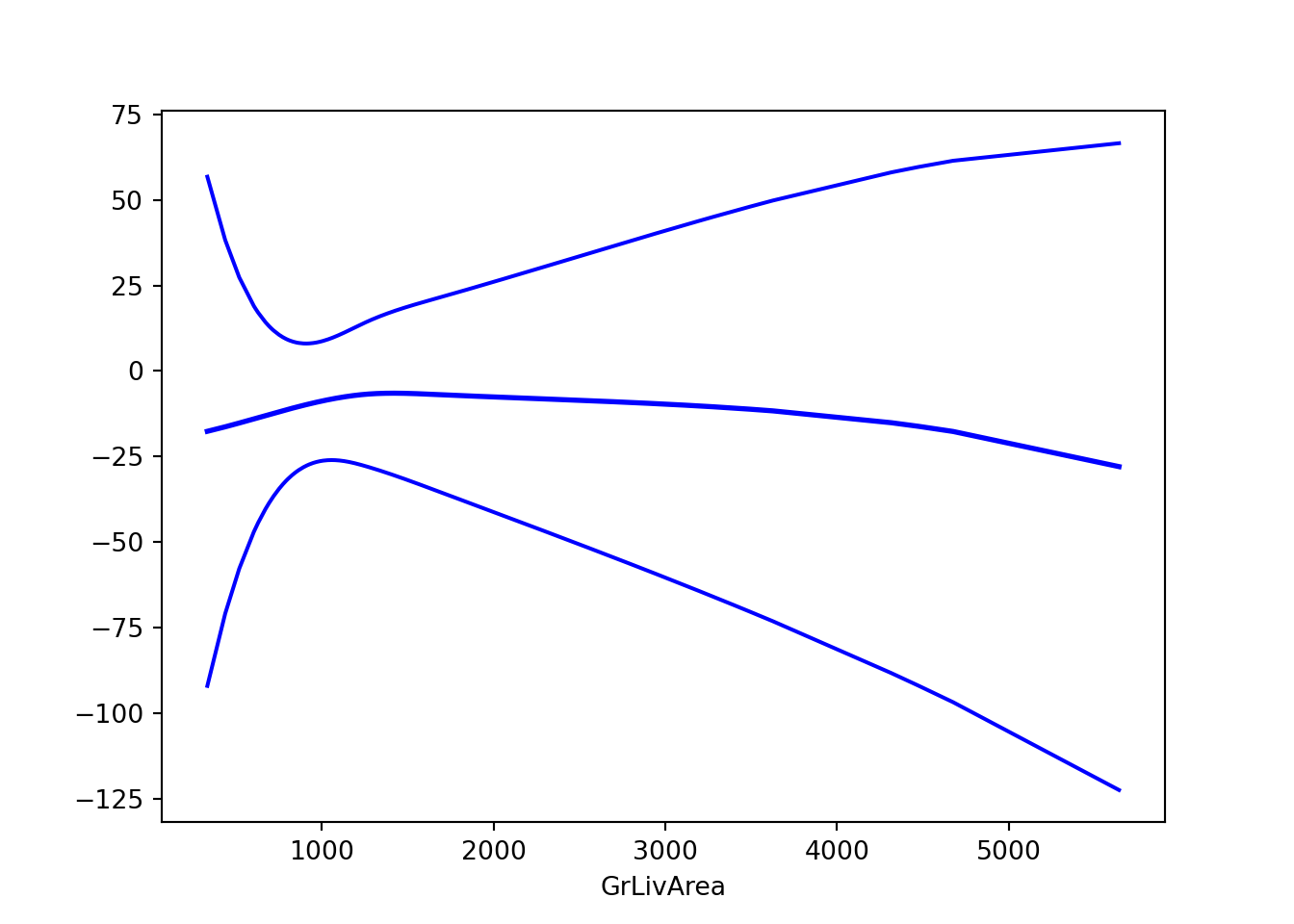
From the plot above, it appears that GrLivArea has three main patterns - below 1250 sqft, between 1250 and 4500 sqft, and above 4500 sqft. But we want bins that are about the same in their effect. Let’s create a new variable along the cut points of < 1250, 1250-4500, 4500+ with the cut function.
Code
import pandas as pd

X_little['GrLivArea_BIN'] = pd.cut(X_little['GrLivArea'], [0, 1250, 4500, 10000])
Now let’s rebuild the logistic regression model with this new categorical version of the GrLivArea variable.
Code
X_little_bin = X_little.drop('GrLivArea', axis = 1)
X_little_bin = pd.get_dummies(X_little_bin, drop_first=True)
X_little_bin = X_little_bin.astype(float)

model_bin = sm.Logit(y, X_little_bin)
result_bin = model_bin.fit()
Optimization terminated successfully.
Current function value: 0.495877
Iterations 8Code
print(result_bin.summary()) Logit Regression Results
==============================================================================
Dep. Variable: bonus No. Observations: 1095
Model: Logit Df Residuals: 1091
Method: MLE Df Model: 3
Date: Sat, 15 Nov 2025 Pseudo R-squ.: 0.2746
Time: 10:54:42 Log-Likelihood: -542.99
converged: True LL-Null: -748.55
Covariance Type: nonrobust LLR p-value: 8.586e-89
===============================================================================================
coef std err z P>|z| [0.025 0.975]
-----------------------------------------------------------------------------------------------
const -6.0360 0.770 -7.835 0.000 -7.546 -4.526
CentralAir_Y 3.2047 0.735 4.362 0.000 1.765 4.645
GrLivArea_BIN_(1250, 4500] 3.3903 0.255 13.312 0.000 2.891 3.889
GrLivArea_BIN_(4500, 10000] 2.8313 1.435 1.973 0.048 0.019 5.644
===============================================================================================From the above output, we can see that GrLivArea_BIN is still a significant variable in our model. The nice part about using a categorical representation for the variable instead of using the GAM for predictions is that we still have some interpretability on this variable using odds ratios for the categories.
For GAMs we can use the gam function in R. Similar to the glm function, you have a model formula to specify the full model. Categorical variables can still be handled with the factor function. The only difference is that we will test the continuous variables with splines to see if those splines produce anything significantly better than their linear representations. The s function is put on every one of the continuous variables. The family = and link = options are used to specify the logistic regression. The method = option is specified here as their are multiple approaches to fitting the GAM in R. We will use the REML approach.
Code
library(mgcv)

fit.gam <- mgcv::gam(bonus ~ s(GrLivArea) + factor(CentralAir),
               data = train, family = binomial(link = 'logit'),
               method = 'REML')
summary(fit.gam)
Family: binomial
Link function: logit

Formula:
bonus ~ s(GrLivArea) + factor(CentralAir)

Parametric coefficients:
                    Estimate Std. Error z value Pr(>|z|)
(Intercept)          -4.9939     0.8200  -6.090 1.13e-09 ***
factor(CentralAir)Y   4.2425     0.8182   5.185 2.16e-07 ***
---
Signif. codes:  0 '***' 0.001 '**' 0.01 '*' 0.05 '.' 0.1 ' ' 1

Approximate significance of smooth terms:
               edf Ref.df Chi.sq p-value
s(GrLivArea) 5.769  6.735  199.8  <2e-16 ***
---
Signif. codes:  0 '***' 0.001 '**' 0.01 '*' 0.05 '.' 0.1 ' ' 1

R-sq.(adj) =  0.438   Deviance explained = 39.9%
-REML = 460.15  Scale est. = 1         n = 1095
Code
plot(fit.gam)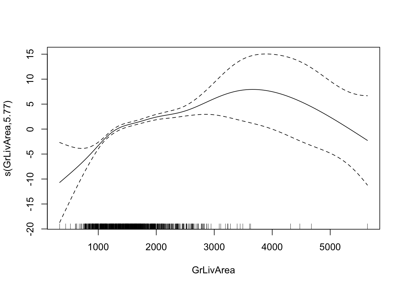
From the above output we can see that GrLivArea and CentralAir are both still significant in this model. However, now the GrLivArea variable is a more complicated transformation. As seen in the graph above, it appears that GrLivArea has a nonlinear pattern with the logit. In fact, the edf (or estimated degrees of freedom) in the output above also shows us this. If the edf value was 1, the best spline was a linear relationship with the target (linearity assumption holds). However, since it is not equal to 1, we cannot say this. How close is close enough to 1? If you wanted a statistical test, we could compare a model with a linear representation of GrLivArea to the spline version with a Likelihood Ratio test.
Code
anova(logit.model, fit.gam, test="LRT")Analysis of Deviance Table
Model 1: bonus ~ GrLivArea + factor(CentralAir)
Model 2: bonus ~ s(GrLivArea) + factor(CentralAir)
Resid. Df Resid. Dev Df Deviance Pr(>Chi)
1 1092.0 968.76
2 1087.2 899.56 4.7692 69.195 1.079e-13 ***
---
Signif. codes: 0 '***' 0.001 '**' 0.01 '*' 0.05 '.' 0.1 ' ' 1The null hypothesis to the above test is that the two models are equal. This null hypothesis would imply that the linearity assumption would hold since the spline is not estimating anything more complicated. However, the p-value was extremely small and therefore the two models are not equal to other. This means that GrLivArea cannot just be modeled linearly with the logit.
From the plot above, it appears that GrLivArea has three main patterns - below 1250 sqft, between 1250 and 4500 sqft, and above 4500 sqft. But we want bins that are about the same in their effect. Let’s create a new variable along the cut points of < 1250, 1250-4500, 4500+ using the cut function.
Code
train <- train %>%
  mutate(GrLivArea_BIN = cut(GrLivArea, breaks = c(-Inf,1250,4500,Inf)))
Now let’s rebuild the logistic regression model with this new categorical version of the GrLivArea variable.
Code
logit.model.bin <- glm(bonus ~ factor(GrLivArea_BIN) + factor(CentralAir),
                       data = train, family = binomial(link = 'logit'))

summary(logit.model.bin)
Call:
glm(formula = bonus ~ factor(GrLivArea_BIN) + factor(CentralAir),
    family = binomial(link = "logit"), data = train)

Coefficients:
                                        Estimate Std. Error z value Pr(>|z|)
(Intercept)                              -6.0360     0.7704  -7.835 4.69e-15
factor(GrLivArea_BIN)(1.25e+03,4.5e+03]   3.3903     0.2547  13.312  < 2e-16
factor(GrLivArea_BIN)(4.5e+03, Inf]       2.8313     1.4349   1.973   0.0485
factor(CentralAir)Y                       3.2047     0.7346   4.362 1.29e-05

(Intercept)                             ***
factor(GrLivArea_BIN)(1.25e+03,4.5e+03] ***
factor(GrLivArea_BIN)(4.5e+03, Inf]     *
factor(CentralAir)Y                     ***
---
Signif. codes:  0 '***' 0.001 '**' 0.01 '*' 0.05 '.' 0.1 ' ' 1

(Dispersion parameter for binomial family taken to be 1)

    Null deviance: 1497.1  on 1094  degrees of freedom
Residual deviance: 1086.0  on 1091  degrees of freedom
AIC: 1094

Number of Fisher Scoring iterations: 6
From the above output, we can see that GrLivArea_BIN is still a significant variable in our model. The nice part about using a categorical representation for the variable instead of using the GAM for predictions is that we still have some interpretability on this variable using odds ratios for the categories.
Predicted Values
Obviously, the predicted logit values really don’t help us too much. Instead we want to gather the predicted probabilities of the target variable categories. Luckily, the software we are looking at make this rather easy to do.
Let’s see how to produce these predicted probabilities in each software!
If you split your data into training and validation (and/or testing) you could score that data set using the predict function. Here we are creating a new data set of 5 observations to score instead. The predict function on the model object (here called result) just needs the dataset to be scored (here called new_ames). By default, the predict function gives the predicted probabilities.
Code
X_little = X[['GrLivArea','CentralAir_Y']]
X_little = sm.add_constant(X_little)

model = sm.Logit(y, X_little)
result = model.fit()
Optimization terminated successfully.
Current function value: 0.442355
Iterations 8Code
print(result.summary()) Logit Regression Results
==============================================================================
Dep. Variable: bonus No. Observations: 1095
Model: Logit Df Residuals: 1092
Method: MLE Df Model: 2
Date: Sat, 15 Nov 2025 Pseudo R-squ.: 0.3529
Time: 10:54:42 Log-Likelihood: -484.38
converged: True LL-Null: -748.55
Covariance Type: nonrobust LLR p-value: 1.868e-115
================================================================================
coef std err z P>|z| [0.025 0.975]
--------------------------------------------------------------------------------
const -11.3561 1.012 -11.222 0.000 -13.339 -9.373
GrLivArea 0.0042 0.000 15.531 0.000 0.004 0.005
CentralAir_Y 4.8704 0.836 5.825 0.000 3.232 6.509
================================================================================Code
new_data = [[1500, 0], [2000, 1], [2250, 1], [2500, 0], [3500, 1]]

new_ames = pd.DataFrame(new_data, columns = ['GrLivArea', 'CentralAir_Y'])
new_ames = sm.add_constant(new_ames)
new_ames = new_ames.astype('float64')

new_ames['Pred'] = result.predict(new_ames)

print(new_ames)
const GrLivArea CentralAir_Y Pred
0 1.0 1500.0 0.0 0.005987
1 1.0 2000.0 1.0 0.862906
2 1.0 2250.0 1.0 0.946864
3 1.0 2500.0 0.0 0.279001
4 1.0 3500.0 1.0 0.999692The print function above looks at the scored data set. Notice that we added an additional column to our original data set we were scoring. This is the predicted probability of a 1. This is default in Python. If you want the predicted probability of the 0 category, you can just subtract this prediction from 1.
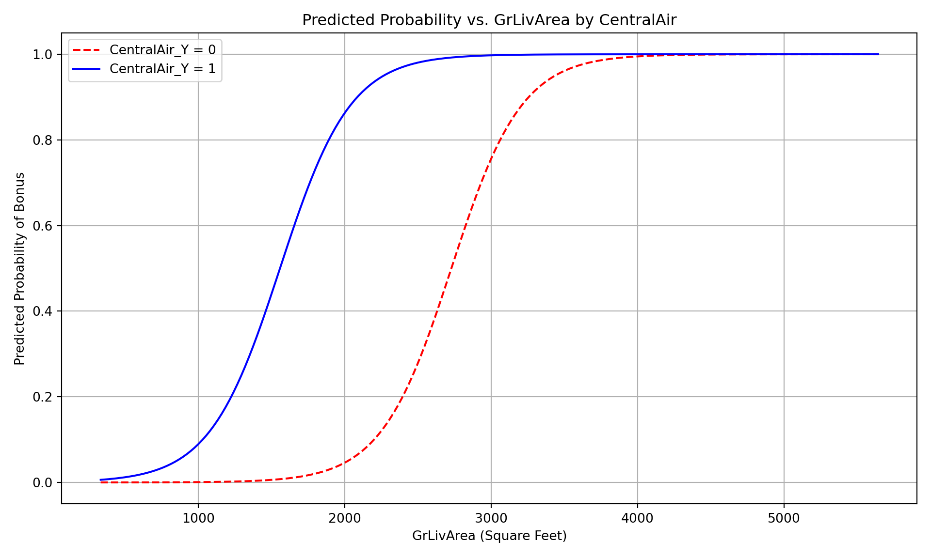
Below we show the effect plot, which will show us the logistic curve across different values of the continuous variable, here GrLivArea. We overlay two of these curves, one for each of the categories of CentralAir. If there is were more continuous variables they are just taken at a specified value - their average value.
If you split your data into training and validation (and/or testing) you could score that data set using the predict function. Here we are creating a new data set of 5 observations to score instead. The predict function has three primary pieces - the model object (here called logit.model, the newdata = option, and the type = option. The newdata = option is where you specify the data set you want scored, while the type = option specifies the type of prediction you want. Here we want the response option since we are predicting the probabilities. If we wanted the predicted logit values we could use the option terms instead.
The visreg function below creates the effect plot, which will show us the logistic curve across different values of the continuous variable, here Gr_Liv_Area. It will show each of the categorical variable categories as a separate curve. If there is were more continuous variables they are just taken at a specified value - their average value.
Code
new_ames <- data.frame(GrLivArea = c(1500, 2000, 2250, 2500, 3500),
                       CentralAir = c("N", "Y", "Y", "N", "Y"))

new_ames <- data.frame(new_ames, 'Pred' = predict(logit.model, newdata = new_ames, type = "response"))

library(visreg)

visreg(logit.model, "GrLivArea", by = "CentralAir", scale = "response",
       overlay = TRUE,
       xlab = 'Greater Living Area (Sqft)',
       ylab = 'Bonus Eligibility')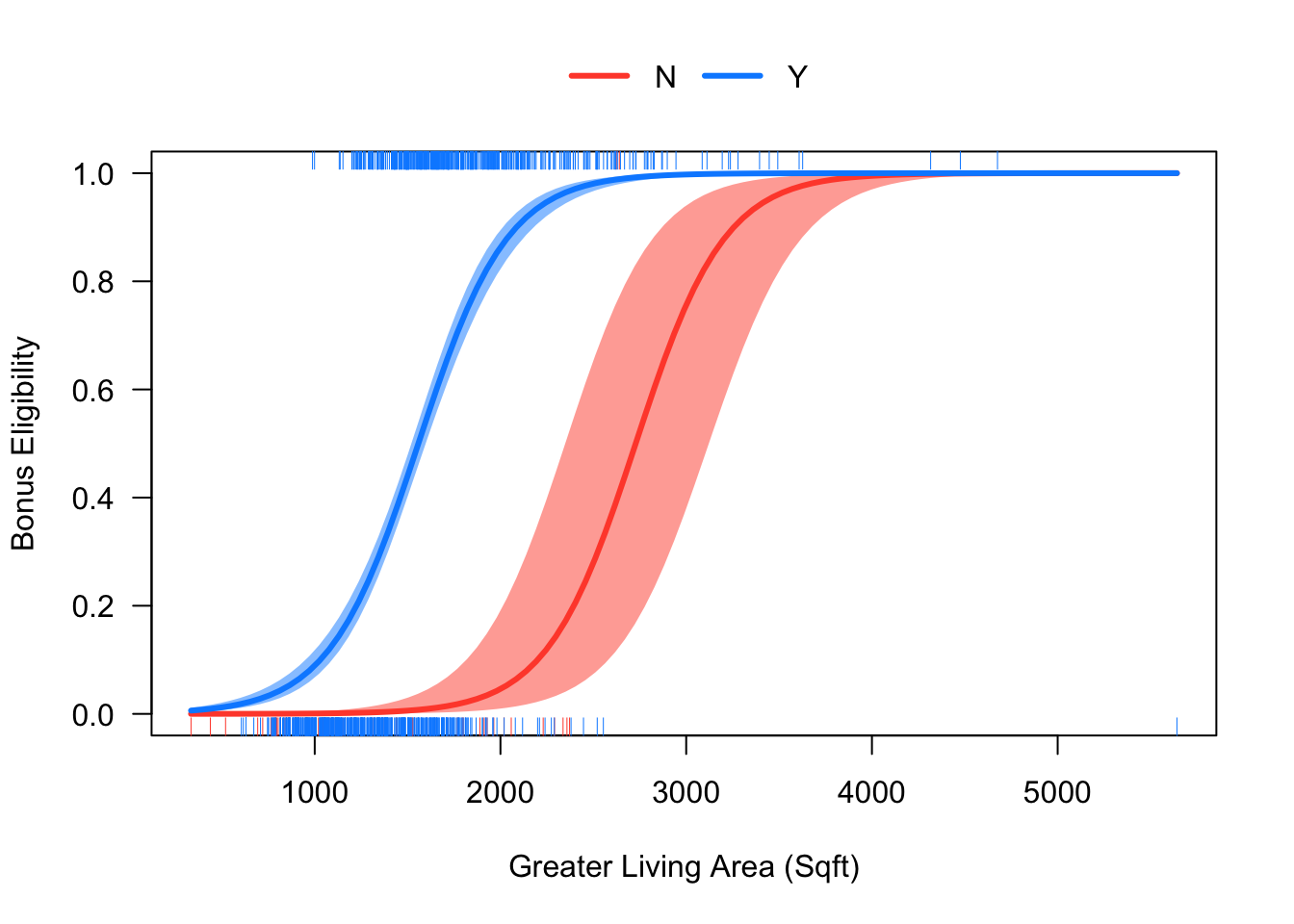
Code
print(new_ames) GrLivArea CentralAir Pred
1 1500 N 0.005987457
2 2000 Y 0.862905502
3 2250 Y 0.946863928
4 2500 N 0.279000584
5 3500 Y 0.999691544The print function above looks at the scored data set. Notice that we added an additional column to our original data set we were scoring. This is the predicted probability of a 1. This is default in R. If you want the predicted probability of the 0 category, you can just subtract this prediction from 1.