Factual information used as a basis for reasoning, discussion, or calculation.
Inference is derived from data. Inference is using information (data) to come to some conclusion. We want to use the information to draw conclusions and make better decisions in the context of our problem. However, the quality of our data drives the quality of our results / inference that arise from any analytics problem. The old saying is that “rotten eggs make a rotten soufflé.” The same applies to any data driven analytics problem. Amazing data professionals with the fanciest machine learning techniques cannot make up for horrible data quality.
First, we need to look at our data before building any models to try and explain/predict our categorical target variable. For this analysis we are going to the popular Ames housing dataset. This dataset contains information on home values for a sample of nearly 1,500 houses in Ames, Iowa in the early 2000s.
To access this data, we first import the fetch_openml function from sklearn.datasets from the popular scikit-learn package. We will also load the pandas package. Using the fetch_openml function with the name = "house_prices" option we have access to the dataset. The head() function will show us a preview of our data.
Code
from sklearn.datasets import fetch_openmlimport pandas as pd# Load Ames Housing datadata = fetch_openml(name ="house_prices", as_frame=True)ames = data.frameames.head()
   Id  MSSubClass MSZoning  ...  SaleType  SaleCondition SalePrice
0   1          60       RL  ...        WD         Normal    208500
1   2          20       RL  ...        WD         Normal    181500
2   3          60       RL  ...        WD         Normal    223500
3   4          70       RL  ...        WD        Abnorml    140000
4   5          60       RL  ...        WD         Normal    250000

[5 rows x 81 columns]
To access this data in R, we would first add the AmesHousing package and create the nicely formatted data with the make_ordinal_ames() function. However, to make sure we get the same results between R and Python, we will just import the dataset from Python to R. After doing that we can use the head() function to show us a preview of the data.
Code
ames <- py$ameshead(ames, n =5)
  Id MSSubClass MSZoning LotFrontage LotArea Street Alley LotShape LandContour
1  1         60       RL          65    8450   Pave  <NA>      Reg         Lvl
2  2         20       RL          80    9600   Pave  <NA>      Reg         Lvl
3  3         60       RL          68   11250   Pave  <NA>      IR1         Lvl
4  4         70       RL          60    9550   Pave  <NA>      IR1         Lvl
5  5         60       RL          84   14260   Pave  <NA>      IR1         Lvl
  Utilities LotConfig LandSlope Neighborhood Condition1 Condition2 BldgType
1    AllPub    Inside       Gtl      CollgCr       Norm       Norm     1Fam
2    AllPub       FR2       Gtl      Veenker      Feedr       Norm     1Fam
3    AllPub    Inside       Gtl      CollgCr       Norm       Norm     1Fam
4    AllPub    Corner       Gtl      Crawfor       Norm       Norm     1Fam
5    AllPub       FR2       Gtl      NoRidge       Norm       Norm     1Fam
  HouseStyle OverallQual OverallCond YearBuilt YearRemodAdd RoofStyle RoofMatl
1     2Story           7           5      2003         2003     Gable  CompShg
2     1Story           6           8      1976         1976     Gable  CompShg
3     2Story           7           5      2001         2002     Gable  CompShg
4     2Story           7           5      1915         1970     Gable  CompShg
5     2Story           8           5      2000         2000     Gable  CompShg
  Exterior1st Exterior2nd MasVnrType MasVnrArea ExterQual ExterCond Foundation
1     VinylSd     VinylSd    BrkFace        196        Gd        TA      PConc
2     MetalSd     MetalSd       None          0        TA        TA     CBlock
3     VinylSd     VinylSd    BrkFace        162        Gd        TA      PConc
4   'Wd Sdng'   'Wd Shng'       None          0        TA        TA     BrkTil
5     VinylSd     VinylSd    BrkFace        350        Gd        TA      PConc
  BsmtQual BsmtCond BsmtExposure BsmtFinType1 BsmtFinSF1 BsmtFinType2
1       Gd       TA           No          GLQ        706          Unf
2       Gd       TA           Gd          ALQ        978          Unf
3       Gd       TA           Mn          GLQ        486          Unf
4       TA       Gd           No          ALQ        216          Unf
5       Gd       TA           Av          GLQ        655          Unf
  BsmtFinSF2 BsmtUnfSF TotalBsmtSF Heating HeatingQC CentralAir Electrical
1          0       150         856    GasA        Ex          Y      SBrkr
2          0       284        1262    GasA        Ex          Y      SBrkr
3          0       434         920    GasA        Ex          Y      SBrkr
4          0       540         756    GasA        Gd          Y      SBrkr
5          0       490        1145    GasA        Ex          Y      SBrkr
  1stFlrSF 2ndFlrSF LowQualFinSF GrLivArea BsmtFullBath BsmtHalfBath FullBath
1      856      854            0      1710            1            0        2
2     1262        0            0      1262            0            1        2
3      920      866            0      1786            1            0        2
4      961      756            0      1717            1            0        1
5     1145     1053            0      2198            1            0        2
  HalfBath BedroomAbvGr KitchenAbvGr KitchenQual TotRmsAbvGrd Functional
1        1            3            1          Gd            8        Typ
2        0            3            1          TA            6        Typ
3        1            3            1          Gd            6        Typ
4        0            3            1          Gd            7        Typ
5        1            4            1          Gd            9        Typ
  Fireplaces FireplaceQu GarageType GarageYrBlt GarageFinish GarageCars
1          0        <NA>     Attchd        2003          RFn          2
2          1          TA     Attchd        1976          RFn          2
3          1          TA     Attchd        2001          RFn          2
4          1          Gd     Detchd        1998          Unf          3
5          1          TA     Attchd        2000          RFn          3
  GarageArea GarageQual GarageCond PavedDrive WoodDeckSF OpenPorchSF
1        548         TA         TA          Y          0          61
2        460         TA         TA          Y        298           0
3        608         TA         TA          Y          0          42
4        642         TA         TA          Y          0          35
5        836         TA         TA          Y        192          84
  EnclosedPorch 3SsnPorch ScreenPorch PoolArea PoolQC Fence MiscFeature MiscVal
1             0         0           0        0   <NA>  <NA>        <NA>       0
2             0         0           0        0   <NA>  <NA>        <NA>       0
3             0         0           0        0   <NA>  <NA>        <NA>       0
4           272         0           0        0   <NA>  <NA>        <NA>       0
5             0         0           0        0   <NA>  <NA>        <NA>       0
  MoSold YrSold SaleType SaleCondition SalePrice
1      2   2008       WD        Normal    208500
2      5   2007       WD        Normal    181500
3      9   2008       WD        Normal    223500
4      2   2006       WD       Abnorml    140000
5     12   2008       WD        Normal    250000
Here are some common considerations when it comes to data before we really get started with heavy analysis:
What to do with missing values?
Do we have the right variables?
How do we reduce the variables we have to a reasonable amount?
Each of those above questions should be thought about and addressed before any real data analysis begins. Let’s explore each of those in more detail.
Missing Values
Missing values are one of the most common problems in real world datasets. However, in their natural form, most (not all) machine learning algorithms cannot handle missing values. If you were to give a typical machine learning algorithm data with missing values it would perform complete case analysis. Complete case analysis is the process of only looking at observations (rows) in your dataset that contain no missing values. This could pose problems. The example below has 80 data points and only 8 missing values scattered throughout it:
Example Data with Missing Values
Although only 10% of all of the data points are missing, the example below shows that only 3 of the 8 observations have no missing values:
Complete Case Analysis
Therefore, even though only 10% of the data points are missing, only 37.5% of all of the data rows would be used to build a model if you wanted to do complete case analysis in the above example. Even if you have millions of observations and had plenty of complete cases, not addressing missing values poses a problem for scoring / predicting new observations that have missing data points.
To address these problems, there are 3 possible solutions:
Delete
Keep
Replace
Deleting Solution
One possible solution to missing values is to delete entire variables that have too many missing values. A common threshold is 50%. If more than half of the observations in a variable are missing, then you should consider removing that variable all together.
Missing Observation Solution - Delete
The business impact of deleting a variable from an analysis should be considered before any variable is deleted. However, if more than half of the observations in a variable are missing, then you might not even know what a majority of that variable truly looks like. This would make imputation (the replace solution to missing values) very questionable as over half of your variable would be generated data and not real.
Keeping Solution
One of the biggest misconceptions around missing values is that they are bad. Missing values are not necessarily bad as they might even be predictive of the outcome. For example, if we were predicting fraudulent claims, missing a home address in demographic information might be a strong predictive signal of fraud.
Categorical variables with missing values are the easiest variables to correct and solve the missing observation problem. If you have a categorical variable with missing values, you should just convert the missing values into their own separate category.
Missing Observations Solution - Keep
By creating a new category in the categorical variable, you do not lose any information. Another possible solution is to replace all missing values in a categorical variable with the most common category. However, this is completely unnecessary as it results in a loss of information.
Replacing Solution
The last common solution to missing observations is replacing these missing values - a process called imputation. As mentioned above, imputation should never be the first option with categorical variables. However, with continuous variables, we cannot just add a new category. With continuous variables we can replace the missing values using a couple of different approaches:
Simple mean / median
Predictive model using other variables
The most common imputation would be replacing the missing values in a variable with a common value of that variable such as the mean or the median of the variable. In a lot of instances this approach is the best approach to imputation.
More recently another approach to imputing missing observations is to use predictive models and other variables to impute the observations. For example, you could use the other predictor variables in your dataset to predict a realistic value for the variable you are imputing. There are some immediate issues that arise from this approach. Multicollinearity (which will be discussed in more detail in the following sections) is a problem with machine learning models where predictor variables are too correlated with each other. By using other variables you to impute values, you are inherently creating a relationship between variables. Unfortunately, only having one variable with missing values in a dataset is quite rare, so a more realistic situation is that many predictor variables are all being used to impute values for each other which further creates high correlation among them. Lastly, a lot of empirical studies have shown that predictive modeling approaches to imputation are no better than the more simplistic mean / median imputation at making machine learning models better at identifying signals in datasets.
In either approach, one additional step is needed - creating a missing flag variable.
Missing Observation Solution - Replace
When imputing continuous variables, we must always create a missing value flag to go along with our newly imputed variable. In the example above, the median of the observations is 32. The two missing observations are imputed with this value. However, we do not want the model to think these are real values of 32 that could also appear in the dataset. We want the model to potentially treat these observations differently and not just think of them as real observations with the value of 32.
Feature Engineering
In the world of machine learning, the importance of good variables cannot be understated. Better variables will always beat fancier modeling techniques. No amount of complicated algorithms can make up for variables that are not predictive. We can help make our variables better through the process of feature engineering.
Feature Engineering
Process of transforming raw data into variables (called features) that are suitable for machine learning models.
How we engineer features in the data completely drives the success of any modeling process that comes afterwards. Good feature engineering involves understanding your data. There are a lot of feature creation programs that will just generate high quantities of features based on common transformations and combinations of your existing variables. However, most of these don’t provide a lot of valuable information since those programs do not understand your data and the context of your business problem.
Let’s work through an example. The following is a common problem in machine learning scenarios to argue for complicated algorithms:
Classic Argument for Fancy Models
In the problem, we have two predictor variables called \(x_1\) and \(x_2\). We are trying to predict which observations are X’s and which are O’s. Some people would argue for fancier machine learning algorithms that can better discover these complicated relationships to identify the difference between the X’s and the O’s. Let’s examine this problem though after some easy feature engineering:
Feature Engineered Variables
The above plot is the same as the previous one, just with new variables. Instead of the original \(x_1\) and \(x_2\) variables, we have used those variables to generate new variables called distance and direction. These variables are the distance from the center of the first plot along with the direction away from the center. Notice in the second plot that it is easy to isolate the X’s from the O’s based solely on an easy cut-off on the distance axis.
Transactional Data
Transactional data contains many different rows of data for each individual in the dataset, typically gathered over time. These types of datasets lend themselves very well to feature engineering.
Model Developed Data vs. Transactional Form
These transactions are rich with information about the individuals in our dataset. There are many different industries where transactional data plays an important role. Some examples include credit card purchasing data, medical and insurance claims data, retail purchasing data, etc. There are some great advantages to transactional data as the data is highly detailed and captures individual behaviors of the customers. This leads to strong correlations in predicting the target variable.
There are some challenges to transactional data due to the complexity and detail they contain. Transactional data can be hard to obtain, process, and store. It also poses problems when it comes to modeling. Most modeling approaches need one line per unique observation, not multiple lines of data. We must aggregate our transactional data for modeling. To not lose the valuable information inside the data, we must creatively engineer features that capture the important information from our transactions.
Summarize categorical variables with counts of transactions in each category, or proportion of observations in each category, as well as the total unique number of categories in a time frame. Of course, all of the continuous variable aggregations could also be calculated for each category as well.
Categorical Feature Engineering
For continuous variables you can think about simple metrics like the average or sum across all transactions. Don’t limit yourself to these basic summaries though. The entire distribution of values provides potentially important information. Perhaps the maximum amount ever spent on a credit card helps, or the interquartile range of transaction amounts.
Continuous Feature Engineering
Those distributional features that are created might also be valuable if broken up into different time ranges for stratification. Instead of just look at all transactions in the dataset, maybe examining the most recent transactions (most recent 30 days for example) would be worthwhile. In fact, a comparison of the most recent transactions compared to the overall trend might prove valuable.
Stratification of Last 30 Days for Transactions
These stratifications can also be done by categories of a variable instead of by time. For example, if a categorical predictor variable has 3 categories (A, B, C) then we can calculate features by each category.
Stratification by Category
Features that summarize changes across time provide value as well. The slope of a trend line through the data describes if the variable is trending up or down. Compare these across different time periods to really see impact. For example, the overall trend may be slightly increasing, but the trend over the past week is actually decreasing.
Features Summarizing Over Time
The best engineered features are ones derived by the creativity of the analytics team working with the data. The value of the modeling comes from the features just as much as the algorithms. Simple aggregations will not suffice. Analytics professionals in this field must think about the business problem at hand and try to engineer features that would describe this. For example, in life insurance fraud, the length of time before a claim is made in which an increase in coverage limit occurs might be important. If a fraudulent claim is about to be made, the fraudster might try to increase the policy coverage limit right before.
Variable Reduction
One of the key struggles of business analytics problems is to reduce the typically immense amounts of variables to a workable list. There are a variety of techniques ranging from rather simple to much more complex:
Common, Basic Techniques:
Business logic / context
Too much missingness
Low (or no) variability
Univariate statistical testing (Section on Model Building)
More Advanced Techniques:
Automatic feature reduction (Section on Model Building)
Regularization (Section on Regularized Regression)
Variable Clustering (Section on Unsupervised Learning)
Business Logic
Even though we are in the world of data analysis and analytics, it doesn’t mean that business logic and knowledge should be left out of the variable reduction process. Good business logic is a quick and easy way to help reduce the number of variables that you have. Common things to remove would be any individual identifiers, information you are not allowed to use, and information you wouldn’t know at decision point, but do after the fact.
Individual identifiers are rarely useful in a modeling context. This is because a new individual in a dataset would never be able to be modeled. In our Ames, Iowa housing dataset, this kind of information would be things like street address. Other examples outside of our dataset would be customer ID’s, social security numbers, phone numbers, etc.
We have to be careful to use information in models that would not be allowed to use. This information would be considered private or protected information that might be illegal to use. For example, gender or race would be protected and not allowed to be used to model whether someone should be given a loan.
Lastly, we should remove any information that would not be known at the point of our business decision making process. For example, if we are trying to model the sale price of a home, we probably will not know what type of sale it would be. Another example would be hoe much money was lost on a defaulted loan when we are modeling if someone should get a loan.
We can use the drop() function on our ames dataframe along with the axis = 1 option to remove the following variables based on business logic. A lot of these are replicated from other variables that repeated information or were numerical categories that represented other categorical variables. We also removed any information from the sale of the home as we are trying to predict the sale price beforehand.
First, we need to load the tidyverse package to make it easier to manipulate data. We can use the select() function on our ames dataframe along with the - in front of the variable to remove the following variables based on business logic. A lot of these are replicated from other variables that repeated information or were numerical categories that represented other categorical variables. We also removed any information from the sale of the home as we are trying to predict the sale price beforehand.
As mentioned above in the section titled Deleting Solution, one possible variable reduction is to remove variables with too much missingness. For our data we will check the count of missing values for each variable. Any variable with more than 730 observations missing will be removed.
We can use the isnull() and sum() functions in conjunction with each other to calculate how many missing values are in each variable. From there we isolate which of the variables have missing value counts over 730. Lastly we print these out in sorted order using the sort_values function.
Code
# Count Missing Valuesmissing_counts = ames.isnull().sum()# More than 50% Missingnessmissing_counts = missing_counts[missing_counts >730]missing_counts.sort_values(ascending =False)
From the above output we can see that 4 variables have missing counts well over 50%. We can then use the drop() function like we have done previously to remove these variables from our dataset.
We can use the is.na() and sapply() functions in conjunction with each other to calculate how many missing values are in each variable. From there we isolate which of the variables have missing value counts over 730. Lastly we print these out in sorted order using the sort function.
Code
# Count missing valuesmissing_counts <-sapply(ames, function(x) sum(is.na(x)))# More than 50% missingness (assuming 730 is 50% of the rows)missing_counts <- missing_counts[missing_counts >730]missing_counts <-sort(missing_counts, decreasing =TRUE)missing_counts
From the above output we can see that 4 variables have missing counts well over 50%. We can then use the select() function like we have done previously to remove these variables from our dataset.
Now that we have removed the variables with too much variability, we can go ahead and perform the “keep” solution to missing values. For all of our categorical variables we can impute missing values with the value of “Missing” as its own, new category.
For categorical variables we will identify all columns that are object or category types using the select_dtypes and columns functions. From there we use the fillna function to fill all the missing values with a new category called 'Missing'.
Code
# Select only categorical columns (object or category dtype)cat_cols = ames.select_dtypes(include=['object', 'category']).columns# Fill missing values with the string "Missing"ames[cat_cols] = ames[cat_cols].fillna('Missing')
For categorical variables we will identify all categorical variables. We identify these variables using the sapply function where we filter variables that are of type is.character or is.factor from our data. We then use the names function to get the specific column names. From there we use the lapply function to fill all the missing values (identified using the is.na() function) with a new category called 'Missing'.
Code
# Select only categorical columns (character or factor)cat_cols <-sapply(ames, function(col) is.character(col) ||is.factor(col))cat_col_names <-names(cat_cols[cat_cols])# Fill missing values in those columns with "Missing"ames[cat_col_names] <-lapply(ames[cat_col_names], function(col) { col[is.na(col)] <-"Missing"return(col)})
We can not yet impute continuous variables because that would involve calculating means and medians on the whole dataset, which is not allowed until we split our data into training and testing subsets.
Low Variability
Another common reason to remove a variable is low or no variability. If a variable has the same value for every observation (no variability) then it cannot be predictive of the target. If a variable never changes, we cannot answer the question, “what happens to our target if our predictor changes?”
The same logic applies to variables with really low variability. For continuous variables, if the variable has a variance less than 0.01 we should consider it removal. For categorical variables, if a variable has 1 category for more than 95% of the data it should be considered for removal. Both of those thresholds are just common thresholds and not set in stone. Your data might require different thresholds. Lastly, business logic around the importance of a variable should always override these thresholds and a variable’s removal.
First, we must separate out our features into continuous and categorical as they have different approaches to identifying low variability. For continuous variables we can use the VarianceThreshold function from the sklearn.feature_selection package. The select_dtypes() function with the include = ['number'] option isolates the numeric variables in our data. We use these numeric variables inside of the fit function of VarianceThreshold once we define our threshold at 0.01. The get_support function identifies the variables that meet the threshold so we want to isolate the variables with the ~ that do not meet the variance threshold and should be removed.
Code
from sklearn.feature_selection import VarianceThresholdames_num = ames.select_dtypes(include = ['number'])# Set your variance threshold threshold =0.01selector = VarianceThreshold(threshold = threshold)selector.fit(ames_num)
VarianceThreshold(threshold=0.01)
In a Jupyter environment, please rerun this cell to show the HTML representation or trust the notebook. On GitHub, the HTML representation is unable to render, please try loading this page with nbviewer.org.
Parameters
threshold
0.01
Code
# Get list of all column namesflag = selector.get_support()all_features = ames_num.columnslow_variability_features = all_features[~flag]print(low_variability_features.tolist())
[]
No variables met this criteria so we will not remove any continuous variables for having too low variability.
For categorical variables we will write a simple for loop where we loop over all variables that are object or category types using the same select_dtypes function as above. For all of these categorical variables we will calculate the proportion of the largest category using the .value_counts(normalize = True).iloc[0] code. The value_counts function with the normalize = True option will return the proportion of each category in descending order. The iloc[0] looks at the first object in this list - the proportion in the highest category. From there we use an if statement to determine if that proportion is greater than 0.95 (or 95%).
Code
# Loop Through Categorical Variables and Look at Top Category %for col in ames.select_dtypes(include=['object', 'category']): top_freq = ames[col].value_counts(normalize=True).iloc[0]if top_freq >0.95:print(f"{col} ({top_freq:.1%})")
Street (99.6%)
Utilities (99.9%)
Heating (97.8%)
Three variables were identified and now we can remove them as we have removed all of the previous ones with the drop() function.
First, we must separate out our features into continuous and categorical as they have different approaches to identifying low variability. For continuous variables we can use the var function in conjunction with the sapply function. The select() and where() functions with the is.numeric function isolates the numeric variables in our data. We use these numeric variables inside of the sapply function. From there we just isolate the names (using the names function) of the variables that are below the threshold of 0.01.
Code
ames_num <- ames %>%select(where(is.numeric))# Set your variance thresholdthreshold <-0.01variances <-sapply(ames_num, var, na.rm =TRUE)low_variability_features <-names(variances[variances < threshold])# Print the low variability featuresprint(low_variability_features)
character(0)
For categorical variables we will write a simple for loop where we loop over all categorical variables. We identify these variables using the names function where we filter (Filter function) variables that are of type is.character or is.factor from our data. For all of these categorical variables we will calculate the proportion of the largest category using the max(prop.table(table(ames[[col]]))) code. The prop.table function along with the table function will return the proportion of each category. We will use the max function to identify the highest proportion. From there we use an if statement to determine if that proportion is greater than 0.95 (or 95%). The cat function both concatenates things and prints them out.
---title: "Data Preparation"format: html: code-fold: show code-tools: trueengine: knitreditor: visual---Instructor: Dr. Aric LaBarr------------------------------------------------------------------------```{r}#| include: false#| warning: false#| error: false#| message: falselibrary(reticulate)reticulate::use_condaenv("wfu_fall_ml", required =TRUE)```# What is/are Data?Data is defined by Merriam Webster as:::: callout-note## DataFactual **information** used as a basis for **reasoning**, **discussion**, or **calculation**.:::Inference is derived from data. Inference is using information (data) to come to some conclusion. We want to use the information to draw conclusions and make better decisions in the context of our problem. However, the quality of our data drives the quality of our results / inference that arise from any analytics problem. The old saying is that "rotten eggs make a rotten soufflé." The same applies to any data driven analytics problem. Amazing data professionals with the fanciest machine learning techniques cannot make up for horrible data quality.First, we need to look at our data before building any models to try and explain/predict our categorical target variable. For this analysis we are going to the popular Ames housing dataset. This dataset contains information on home values for a sample of nearly 1,500 houses in Ames, Iowa in the early 2000s.Let's see how to do this in each of our software!::: {.panel-tabset .nav-pills}## PythonTo access this data, we first import the `fetch_openml` function from `sklearn.datasets` from the popular `scikit-learn` package. We will also load the `pandas` package. Using the `fetch_openml` function with the `name = "house_prices"` option we have access to the dataset. The `head()` function will show us a preview of our data.```{python}#| warning: false#| error: false#| message: falsefrom sklearn.datasets import fetch_openmlimport pandas as pd# Load Ames Housing datadata = fetch_openml(name ="house_prices", as_frame=True)ames = data.frameames.head()```## RTo access this data in R, we would first add the `AmesHousing` package and create the nicely formatted data with the `make_ordinal_ames()` function. However, to make sure we get the same results between R and Python, we will just import the dataset from Python to R. After doing that we can use the `head()` function to show us a preview of the data.```{r}#| warning: false#| error: false#| message: falseames <- py$ameshead(ames, n =5)```:::Here are some common considerations when it comes to data before we really get started with heavy analysis:- What to do with missing values?- Do we have the right variables?- How do we reduce the variables we have to a reasonable amount?Each of those above questions should be thought about and addressed before any real data analysis begins. Let's explore each of those in more detail.# Missing ValuesMissing values are one of the most common problems in real world datasets. However, in their natural form, most (not all) machine learning algorithms cannot handle missing values. If you were to give a typical machine learning algorithm data with missing values it would perform **complete case analysis**. Complete case analysis is the process of only looking at observations (rows) in your dataset that contain no missing values. This could pose problems. The example below has 80 data points and only 8 missing values scattered throughout it: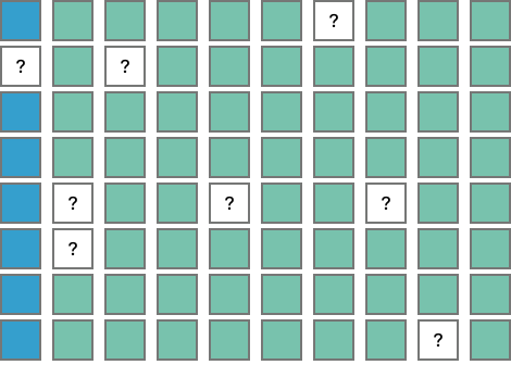{fig-align="center" width="4.9in"}Although only 10% of all of the data points are missing, the example below shows that only 3 of the 8 observations have no missing values: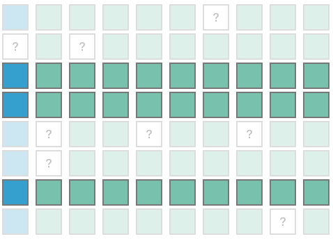{fig-align="center" width="4.98in"}Therefore, even though only 10% of the data points are missing, only 37.5% of all of the data rows would be used to build a model if you wanted to do complete case analysis in the above example. Even if you have millions of observations and had plenty of complete cases, not addressing missing values poses a problem for scoring / predicting new observations that have missing data points.To address these problems, there are 3 possible solutions:1. Delete2. Keep3. Replace## Deleting SolutionOne possible solution to missing values is to delete entire variables that have too many missing values. A common threshold is 50%. If more than half of the observations in a variable are missing, then you should **consider** removing that variable all together.{fig-align="center" width="0.94in"}The business impact of deleting a variable from an analysis should be considered before any variable is deleted. However, if more than half of the observations in a variable are missing, then you might not even know what a majority of that variable truly looks like. This would make imputation (the replace solution to missing values) very questionable as over half of your variable would be generated data and not real.## Keeping Solution {#keeping-solution}One of the biggest misconceptions around missing values is that they are bad. Missing values are not necessarily bad as they might even be predictive of the outcome. For example, if we were predicting fraudulent claims, missing a home address in demographic information might be a strong predictive signal of fraud.Categorical variables with missing values are the easiest variables to correct and solve the missing observation problem. If you have a categorical variable with missing values, you should just convert the missing values into their own separate category.{fig-align="center" width="4.06in"}By creating a new category in the categorical variable, you do not lose any information. Another possible solution is to replace all missing values in a categorical variable with the most common category. However, this is completely unnecessary as it results in a loss of information.## Replacing SolutionThe last common solution to missing observations is replacing these missing values - a process called **imputation**. As mentioned above, imputation should never be the first option with categorical variables. However, with continuous variables, we cannot just add a new category. With continuous variables we can replace the missing values using a couple of different approaches:1. Simple mean / median2. Predictive model using other variablesThe most common imputation would be replacing the missing values in a variable with a common value of that variable such as the mean or the median of the variable. In a lot of instances this approach is the best approach to imputation.More recently another approach to imputing missing observations is to use predictive models and other variables to impute the observations. For example, you could use the other predictor variables in your dataset to predict a realistic value for the variable you are imputing. There are some immediate issues that arise from this approach. Multicollinearity (which will be discussed in more detail in the following sections) is a problem with machine learning models where predictor variables are too correlated with each other. By using other variables you to impute values, you are inherently creating a relationship between variables. Unfortunately, only having one variable with missing values in a dataset is quite rare, so a more realistic situation is that many predictor variables are all being used to impute values for each other which further creates high correlation among them. Lastly, a lot of empirical studies have shown that predictive modeling approaches to imputation are no better than the more simplistic mean / median imputation at making machine learning models better at identifying signals in datasets.In either approach, one additional step is needed - creating a missing flag variable.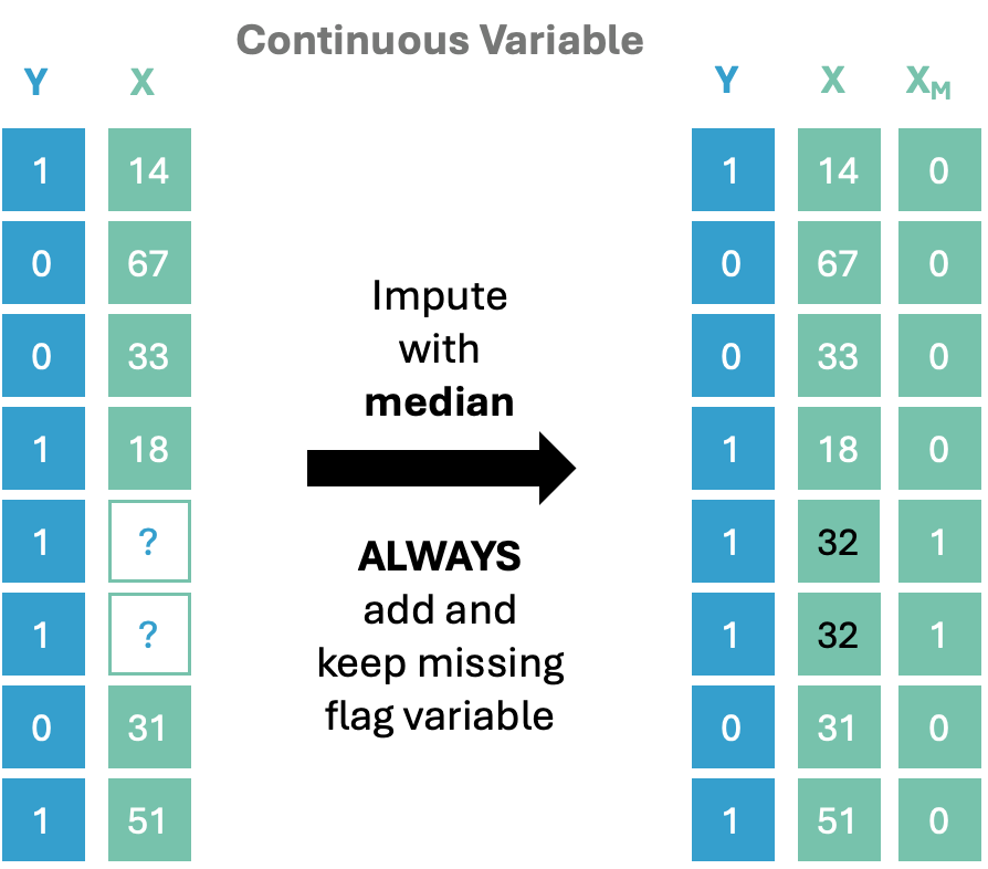{fig-align="center" width="4.55in"}When imputing continuous variables, we must always create a missing value flag to go along with our newly imputed variable. In the example above, the median of the observations is 32. The two missing observations are imputed with this value. However, we do not want the model to think these are real values of 32 that could also appear in the dataset. We want the model to potentially treat these observations differently and not just think of them as real observations with the value of 32.# Feature EngineeringIn the world of machine learning, the importance of good variables cannot be understated. Better variables will always beat fancier modeling techniques. No amount of complicated algorithms can make up for variables that are not predictive. We can help make our variables better through the process of **feature engineering**.::: callout-note## Feature EngineeringProcess of transforming raw data into variables (called **features**) that are suitable for machine learning models.:::How we engineer features in the data completely drives the success of any modeling process that comes afterwards. Good feature engineering involves understanding your data. There are a lot of feature creation programs that will just generate high quantities of features based on common transformations and combinations of your existing variables. However, most of these don't provide a lot of valuable information since those programs do not understand your data and the context of your business problem.Let's work through an example. The following is a common problem in machine learning scenarios to argue for complicated algorithms:{fig-align="center" width="5.71in"}In the problem, we have two predictor variables called $x_1$ and $x_2$. We are trying to predict which observations are X's and which are O's. Some people would argue for fancier machine learning algorithms that can better discover these complicated relationships to identify the difference between the X's and the O's. Let's examine this problem though after some easy feature engineering:{fig-align="center" width="5.64in"}The above plot is the same as the previous one, just with new variables. Instead of the original $x_1$ and $x_2$ variables, we have used those variables to generate new variables called *distance* and *direction*. These variables are the distance from the center of the first plot along with the direction away from the center. Notice in the second plot that it is easy to isolate the X's from the O's based solely on an easy cut-off on the *distance* axis.## Transactional DataTransactional data contains many different rows of data for each individual in the dataset, typically gathered over time. These types of datasets lend themselves very well to feature engineering.{fig-align="center" width="6.18in"}These transactions are rich with information about the individuals in our dataset. There are many different industries where transactional data plays an important role. Some examples include credit card purchasing data, medical and insurance claims data, retail purchasing data, etc. There are some great advantages to transactional data as the data is highly detailed and captures individual behaviors of the customers. This leads to strong correlations in predicting the target variable.There are some challenges to transactional data due to the complexity and detail they contain. Transactional data can be hard to obtain, process, and store. It also poses problems when it comes to modeling. Most modeling approaches need one line per unique observation, not multiple lines of data. We must aggregate our transactional data for modeling. To not lose the valuable information inside the data, we must creatively engineer features that capture the important information from our transactions.Summarize categorical variables with counts of transactions in each category, or proportion of observations in each category, as well as the total unique number of categories in a time frame. Of course, all of the continuous variable aggregations could also be calculated for each category as well.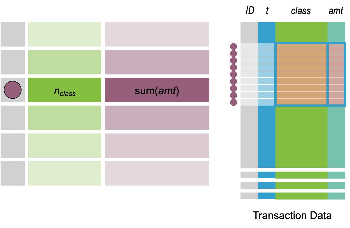{fig-align="center" width="6.13in"}For continuous variables you can think about simple metrics like the average or sum across all transactions. Don't limit yourself to these basic summaries though. The entire distribution of values provides potentially important information. Perhaps the maximum amount ever spent on a credit card helps, or the interquartile range of transaction amounts.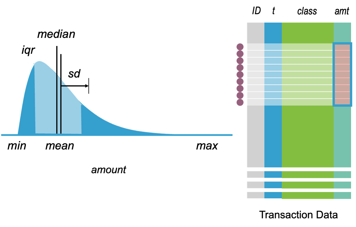{fig-align="center" width="6.25in"}Those distributional features that are created might also be valuable if broken up into different time ranges for stratification. Instead of just look at all transactions in the dataset, maybe examining the most recent transactions (most recent 30 days for example) would be worthwhile. In fact, a comparison of the most recent transactions compared to the overall trend might prove valuable.{fig-align="center" width="6.22in"}These stratifications can also be done by categories of a variable instead of by time. For example, if a categorical predictor variable has 3 categories (A, B, C) then we can calculate features by each category.{fig-align="center" width="6.25in"}Features that summarize changes across time provide value as well. The slope of a trend line through the data describes if the variable is trending up or down. Compare these across different time periods to really see impact. For example, the overall trend may be slightly increasing, but the trend over the past week is actually decreasing.{fig-align="center" width="6.4in"}The best engineered features are ones derived by the creativity of the analytics team working with the data. The value of the modeling comes from the features just as much as the algorithms. Simple aggregations will not suffice. Analytics professionals in this field must think about the business problem at hand and try to engineer features that would describe this. For example, in life insurance fraud, the length of time before a claim is made in which an increase in coverage limit occurs might be important. If a fraudulent claim is about to be made, the fraudster might try to increase the policy coverage limit right before.# Variable ReductionOne of the key struggles of business analytics problems is to reduce the typically immense amounts of variables to a workable list. There are a variety of techniques ranging from rather simple to much more complex:- Common, Basic Techniques: - Business logic / context - Too much missingness - Low (or no) variability - Univariate statistical testing (Section on [Model Building](part_2_model))- More Advanced Techniques: - Automatic feature reduction (Section on Model Building) - Regularization (Section on Regularized Regression) - Variable Clustering (Section on Unsupervised Learning)## Business LogicEven though we are in the world of data analysis and analytics, it doesn't mean that business logic and knowledge should be left out of the variable reduction process. Good business logic is a quick and easy way to help reduce the number of variables that you have. Common things to remove would be any individual identifiers, information you are not allowed to use, and information you wouldn't know at decision point, but do after the fact.Individual identifiers are rarely useful in a modeling context. This is because a new individual in a dataset would never be able to be modeled. In our Ames, Iowa housing dataset, this kind of information would be things like *street address*. Other examples outside of our dataset would be customer ID's, social security numbers, phone numbers, etc.We have to be careful to use information in models that would not be allowed to use. This information would be considered private or protected information that might be illegal to use. For example, gender or race would be protected and not allowed to be used to model whether someone should be given a loan.Lastly, we should remove any information that would not be known at the point of our business decision making process. For example, if we are trying to model the sale price of a home, we probably will not know what type of sale it would be. Another example would be hoe much money was lost on a defaulted loan when we are modeling if someone should get a loan.Let's remove some variables in each of software!::: {.panel-tabset .nav-pills}## PythonWe can use the `drop()` function on our `ames` dataframe along with the `axis = 1` option to remove the following variables based on business logic. A lot of these are replicated from other variables that repeated information or were numerical categories that represented other categorical variables. We also removed any information from the sale of the home as we are trying to predict the sale price beforehand.```{python}#| warning: false#| error: false#| message: false# Remove Variables with Business Logicames = ames.drop(['Id', 'MSSubClass', 'Functional', 'MSZoning', 'Neighborhood', 'LandSlope', 'Condition2','OverallCond', 'RoofStyle', 'RoofMatl', 'Exterior1st','Exterior2nd', 'MasVnrType', 'MasVnrArea', 'ExterCond','BsmtCond', 'BsmtExposure', 'BsmtFinType1', 'BsmtFinSF1','BsmtFinType2', 'BsmtFinSF2', 'BsmtUnfSF', 'Electrical','LowQualFinSF', 'BsmtFullBath', 'BsmtHalfBath','KitchenAbvGr', 'GarageFinish', 'SaleType', 'SaleCondition'], axis =1)```## RFirst, we need to load the `tidyverse` package to make it easier to manipulate data. We can use the `select()` function on our `ames` dataframe along with the `-` in front of the variable to remove the following variables based on business logic. A lot of these are replicated from other variables that repeated information or were numerical categories that represented other categorical variables. We also removed any information from the sale of the home as we are trying to predict the sale price beforehand.```{r}#| warning: false#| error: false#| message: falselibrary(tidyverse)ames <- ames %>%select(-Id, -MSSubClass, -Functional, -MSZoning, -Neighborhood, -LandSlope, -Condition2,-OverallCond, -RoofStyle, -RoofMatl, -Exterior1st,-Exterior2nd, -MasVnrType, -MasVnrArea, -ExterCond,-BsmtCond, -BsmtExposure, -BsmtFinType1, -BsmtFinSF1,-BsmtFinType2, -BsmtFinSF2, -BsmtUnfSF, -Electrical,-LowQualFinSF, -BsmtFullBath, -BsmtHalfBath,-KitchenAbvGr, -GarageFinish, -SaleType, -SaleCondition )```:::## MissingnessAs mentioned above in the section titled Deleting Solution, one possible variable reduction is to remove variables with too much missingness. For our data we will check the count of missing values for each variable. Any variable with more than 730 observations missing will be removed.Let's see how to do this in each of our software!::: {.panel-tabset .nav-pills}## PythonWe can use the `isnull()` and `sum()` functions in conjunction with each other to calculate how many missing values are in each variable. From there we isolate which of the variables have missing value counts over 730. Lastly we print these out in sorted order using the `sort_values` function.```{python}#| warning: false#| error: false#| message: false# Count Missing Valuesmissing_counts = ames.isnull().sum()# More than 50% Missingnessmissing_counts = missing_counts[missing_counts >730]missing_counts.sort_values(ascending =False)```From the above output we can see that 4 variables have missing counts well over 50%. We can then use the `drop()` function like we have done previously to remove these variables from our dataset.```{python}#| warning: false#| error: false#| message: false# Remove Variables with Missingnessames = ames.drop(['PoolQC', 'MiscFeature', 'Alley', 'Fence'], axis =1)```## RWe can use the `is.na()` and `sapply()` functions in conjunction with each other to calculate how many missing values are in each variable. From there we isolate which of the variables have missing value counts over 730. Lastly we print these out in sorted order using the `sort` function.```{r}#| warning: false#| error: false#| message: false# Count missing valuesmissing_counts <-sapply(ames, function(x) sum(is.na(x)))# More than 50% missingness (assuming 730 is 50% of the rows)missing_counts <- missing_counts[missing_counts >730]missing_counts <-sort(missing_counts, decreasing =TRUE)missing_counts```From the above output we can see that 4 variables have missing counts well over 50%. We can then use the `select()` function like we have done previously to remove these variables from our dataset.```{r}#| warning: false#| error: false#| message: falseames <- ames %>%select(-PoolQC, -MiscFeature, -Alley, -Fence )```:::Now that we have removed the variables with too much variability, we can go ahead and perform the ["keep"](part_1_intro#keeping-solution) solution to missing values. For all of our categorical variables we can impute missing values with the value of "Missing" as its own, new category.Let's see how to do this in each of our software!::: {.panel-tabset .nav-pills}## PythonFor categorical variables we will identify all columns that are `object` or `category` types using the `select_dtypes` and `columns` functions. From there we use the `fillna` function to fill all the missing values with a new category called `'Missing'`.```{python}#| warning: false#| error: false#| message: false# Select only categorical columns (object or category dtype)cat_cols = ames.select_dtypes(include=['object', 'category']).columns# Fill missing values with the string "Missing"ames[cat_cols] = ames[cat_cols].fillna('Missing')```## RFor categorical variables we will identify all categorical variables. We identify these variables using the `sapply` function where we filter variables that are of type `is.character` or `is.factor` from our data. We then use the `names` function to get the specific column names. From there we use the `lapply` function to fill all the missing values (identified using the `is.na()` function) with a new category called `'Missing'`.```{r}#| warning: false#| error: false#| message: false# Select only categorical columns (character or factor)cat_cols <-sapply(ames, function(col) is.character(col) ||is.factor(col))cat_col_names <-names(cat_cols[cat_cols])# Fill missing values in those columns with "Missing"ames[cat_col_names] <-lapply(ames[cat_col_names], function(col) { col[is.na(col)] <-"Missing"return(col)})```:::We can **not** yet impute continuous variables because that would involve calculating means and medians on the whole dataset, which is not allowed until we split our data into training and testing subsets.## Low VariabilityAnother common reason to remove a variable is low or no variability. If a variable has the same value for every observation (no variability) then it cannot be predictive of the target. If a variable never changes, we cannot answer the question, "what happens to our target if our predictor changes?"The same logic applies to variables with really low variability. For continuous variables, if the variable has a variance less than 0.01 we should consider it removal. For categorical variables, if a variable has 1 category for more than 95% of the data it should be considered for removal. Both of those thresholds are just common thresholds and not set in stone. Your data might require different thresholds. Lastly, business logic around the importance of a variable should **always** override these thresholds and a variable's removal.Let's see how to do this in each of our software!::: {.panel-tabset .nav-pills}## PythonFirst, we must separate out our features into continuous and categorical as they have different approaches to identifying low variability. For continuous variables we can use the `VarianceThreshold` function from the `sklearn.feature_selection` package. The `select_dtypes()` function with the `include = ['number']` option isolates the numeric variables in our data. We use these numeric variables inside of the `fit` function of `VarianceThreshold` once we define our threshold at `0.01`. The `get_support` function identifies the variables that **meet** the threshold so we want to isolate the variables with the `~` that do not meet the variance threshold and should be removed.```{python}#| warning: false#| error: false#| message: falsefrom sklearn.feature_selection import VarianceThresholdames_num = ames.select_dtypes(include = ['number'])# Set your variance threshold threshold =0.01selector = VarianceThreshold(threshold = threshold)selector.fit(ames_num)# Get list of all column namesflag = selector.get_support()all_features = ames_num.columnslow_variability_features = all_features[~flag]print(low_variability_features.tolist())```No variables met this criteria so we will not remove any continuous variables for having too low variability.For categorical variables we will write a simple `for` loop where we loop over all variables that are `object` or `category` types using the same `select_dtypes` function as above. For all of these categorical variables we will calculate the proportion of the largest category using the `.value_counts(normalize = True).iloc[0]` code. The `value_counts` function with the `normalize = True` option will return the proportion of each category in descending order. The `iloc[0]` looks at the first object in this list - the proportion in the highest category. From there we use an `if` statement to determine if that proportion is greater than 0.95 (or 95%).```{python}#| warning: false#| error: false#| message: false# Loop Through Categorical Variables and Look at Top Category %for col in ames.select_dtypes(include=['object', 'category']): top_freq = ames[col].value_counts(normalize=True).iloc[0]if top_freq >0.95:print(f"{col} ({top_freq:.1%})")```Three variables were identified and now we can remove them as we have removed all of the previous ones with the `drop()` function.```{python}#| warning: false#| error: false#| message: false# Remove Variables with Low Variabilityames = ames.drop(['Street', 'Utilities', 'Heating'], axis =1)```## RFirst, we must separate out our features into continuous and categorical as they have different approaches to identifying low variability. For continuous variables we can use the `var` function in conjunction with the `sapply` function. The `select()` and `where()` functions with the `is.numeric` function isolates the numeric variables in our data. We use these numeric variables inside of the `sapply` function. From there we just isolate the names (using the `names` function) of the variables that are below the threshold of `0.01`.```{r}#| warning: false#| error: false#| message: falseames_num <- ames %>%select(where(is.numeric))# Set your variance thresholdthreshold <-0.01variances <-sapply(ames_num, var, na.rm =TRUE)low_variability_features <-names(variances[variances < threshold])# Print the low variability featuresprint(low_variability_features)```For categorical variables we will write a simple `for` loop where we loop over all categorical variables. We identify these variables using the `names` function where we filter (`Filter` function) variables that are of type `is.character` or `is.factor` from our data. For all of these categorical variables we will calculate the proportion of the largest category using the `max(prop.table(table(ames[[col]])))` code. The `prop.table` function along with the `table` function will return the proportion of each category. We will use the `max` function to identify the highest proportion. From there we use an `if` statement to determine if that proportion is greater than 0.95 (or 95%). The `cat` function both concatenates things and prints them out.```{r}#| warning: false#| error: false#| message: falsecat_cols <-names(Filter(function(x) is.character(x) ||is.factor(x), ames))for (col in cat_cols) { top_freq <-max(prop.table(table(ames[[col]])))if (top_freq >0.95) {cat(sprintf("%s (%.1f%%)\n", col, top_freq *100)) }}```Three variables were identified and now we can remove them as we have removed all of the previous ones with the `select()` function.```{r}#| warning: false#| error: false#| message: falseames <- ames %>%select(-Street, -Utilities, -Heating )```:::











