In mathematics and statistics, there are popular theories involving distributions of known values. The Central Limit Theorem is one of them. We don’t need complicated mathematics for us to approximate distributional assumptions when we use simulations. This is especially helpful when finding a closed form solution is very difficult, if not impossible. A closed form solution to a mathematical/statistical distribution problem means that you can mathematically calculate the distribution through equations. Real world data can be very complicated and may change based on different inputs which each have their own unique distribution. Simulation can reveal an approximation of these output distributions.
The next two sections work through some examples of this.
Central Limit Theorem
Assume you do not know the Central Limit Theorem, but want to study and understand the sampling distribution of sample means. You take samples of size 10, 50, and 100 from the following three population distributions and calculate the sample means repeatedly:
Normal distribution
Uniform distribution
Exponential distribution
Let’s use our software to simulate the sampling distributions of sample means across each of the above distributions and sample sizes!
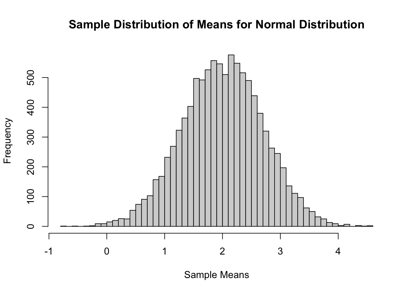
This simulation can easily be done in R without the use of loops. First, we set the sample size and simulation size of the simulation. Next, we just randomly sample from each of the above distributions using the rnorm, runif, and rexp functions. In each of these functions we sample as many observations we would need across all simulations which is the product of the sample size with the simulation size. We then use the matrix function to take the draws from the random sampling functions and allocate the observations across rows and columns of a matrix. Specifically, we will use the rows as simulations, and columns as samples. Lastly, we just use the apply function for each matrix and apply the mean function to each row (or simulation). From there we can plot the distributions of the sample means.
Code
sample.size <-50simulation.size <-10000X1 <-matrix(data=rnorm(n=(sample.size*simulation.size), mean=2, sd=5), nrow=simulation.size, ncol=sample.size, byrow=TRUE)X2 <-matrix(data=runif(n=(sample.size*simulation.size), min=5, max=105), nrow=simulation.size, ncol=sample.size, byrow=TRUE)X3 <-matrix(data=(rexp(n=(sample.size*simulation.size)) +3), nrow=simulation.size, ncol=sample.size, byrow=TRUE)Mean.X1 <-apply(X1,1,mean)Mean.X2 <-apply(X2,1,mean)Mean.X3 <-apply(X3,1,mean)hist(Mean.X1, breaks=50, main='Sample Distribution of Means for Normal Distribution', xlab='Sample Means')
Code
hist(Mean.X2, breaks=50, main='Sample Distribution of Means for Uniform Distribution', xlab='Sample Means')
Code
hist(Mean.X3, breaks=50, main='Sample Distribution of Means for Exponential Distribution', xlab='Sample Means')
The example above shows sampling distributions for the mean when the sample size is 50. Easily changing that piece of the code will allow the user to see these sampling distributions at different sample sizes.
As you can see above, the sampling distribution for the sample means is approximately normally distributed, regardless of the population distribution, as long as the sample size is big enough.
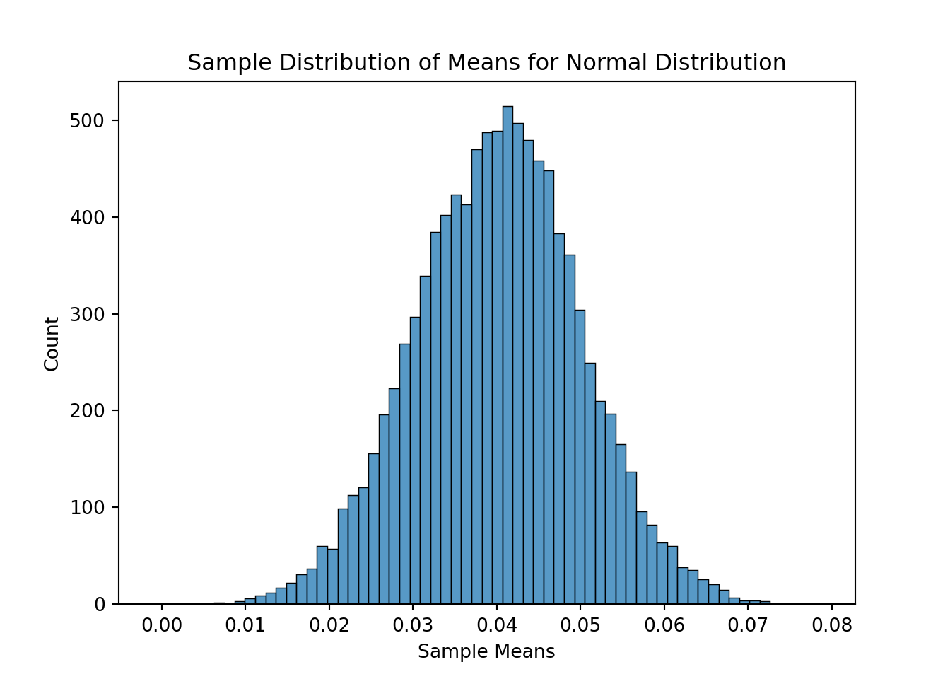
This simulation can easily be done in Python without the use of loops. First, we set the sample size and simulation size of the simulation. Next, we just randomly sample from each of the above distributions using the random.normal, random.uniform, and random.exponential functions from numpy. In each of these functions we sample as many observations we would need across all simulations which is the product of the sample size with the simulation size. We then use the reshape function on these arrays to take the draws from the random sampling functions and allocate the observations across rows and columns of an array. Specifically, we will use the rows as simulations, and columns as samples. Lastly, we just use the mean function for each array and apply the axis = 1 option to each row (or simulation). From there we can plot the distributions of the sample means.
import seaborn as snsimport matplotlib.pyplot as pltax = sns.histplot(data = Mean_X1)ax.set_title('Sample Distribution of Means for Normal Distribution')ax.set_xlabel("Sample Means")
Code
ax = sns.histplot(data = Mean_X2)ax.set_title('Sample Distribution of Means for Uniform Distribution')ax.set_xlabel("Sample Means")
Code
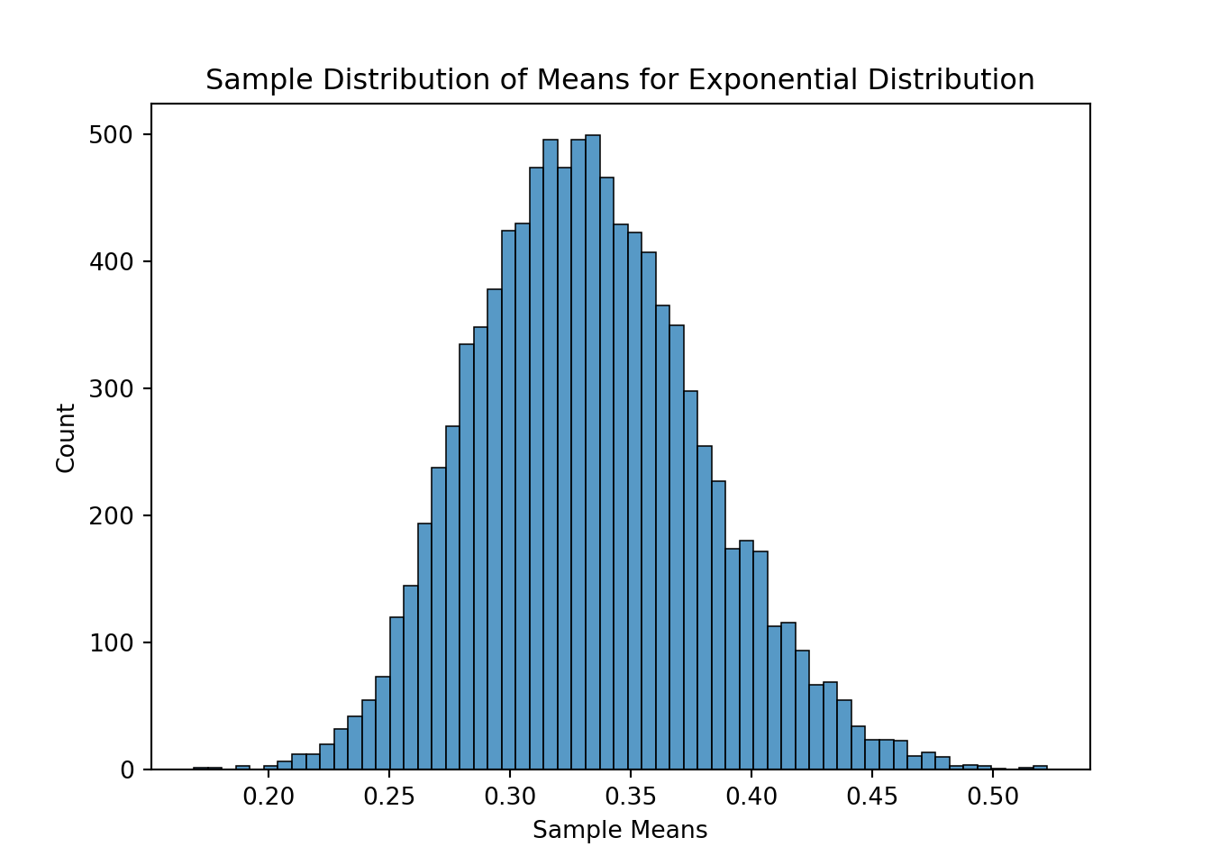
ax = sns.histplot(data = Mean_X3)ax.set_title('Sample Distribution of Means for Exponential Distribution')ax.set_xlabel("Sample Means")
The example above shows sampling distributions for the mean when the sample size is 50. Easily changing that piece of the code will allow the user to see these sampling distributions at different sample sizes.
As you can see above, the sampling distribution for the sample means is approximately normally distributed, regardless of the population distribution, as long as the sample size is big enough.
This simulation can easily be done in SAS with a couple of loops in a DATA step. First, we set the sample size and simulation size of the simulation with MACRO variables using the % symbol. Next, we open two DO loops to loop over the simulation and sample size. Then we just randomly sample from each of the above distributions using the RAND function with the Normal, Uniform, and Exponential options. We then use the OUTPUT statement to make sure that the results from each iteration in the loop are stored as a separate row in the dataset. Lastly, we just use the PROC MEANS procedure to calculate the means across each variable (using the VAR statement) for each simulation (using the BY statement). We use the OUTPUT statement and OUT option to store the resulting means into separate datasets as different columns - one column for each simulation. From there we can plot the distributions of the sample means using three separate SGPLOT procedure calls.
Code
%let Sample_Size =50;%let Simulation_Size =10000;data CLT; do sim =1 to &Simulation_Size; do obs =1 to &Sample_Size; call streaminit(12345); X1 =RAND('Normal', 2, 5); X2 =5+100*RAND('Uniform'); X3 =3+RAND('Exponential'); output; end; end;run;proc means data=CLT noprint mean; var X1 X2 X3; by sim; output out=Means mean(X1 X2 X3)=Mean_X1 Mean_X2 Mean_X3;run;proc sgplot data=Means; title 'Sampling Distribution of Means'; title2 'Normal Distribution'; histogram Mean_X1; keylegend / location=inside position=topright;run;proc sgplot data=Means; title 'Sampling Distribution of Means'; title2 'Uniform Distribution'; histogram Mean_X2; keylegend / location=inside position=topright;run;proc sgplot data=Means; title 'Sampling Distribution of Means'; title2 'Exponential Distribution'; histogram Mean_X3; keylegend / location=inside position=topright;run;
The example above shows sampling distributions for the mean when the sample size is 50. Easily changing that piece of the code will allow the user to see these sampling distributions at different sample sizes.
As you can see above, the sampling distribution for the sample means is approximately normally distributed, regardless of the population distribution, as long as the sample size is big enough.
Omitted Variable Bias
What if you leave an important variable out of a linear regression that should have been in the model? From statistical theory it would change the bias of the coefficients in the model as well as the variability of the coefficients, depending on if the variable left out was correlated with another variable in the model. Simulation can help us show this as well as determine how bad these problems could get under different circumstances.
Let’s simulate the following regression model:
\[
Y = -13 + 1.21X_1 + 3.45X_2 + \varepsilon
\]
Assume that the errors, \(\varepsilon\) , in the model above are normally distributed with a mean of 0 and standard deviation of 1.5. Also assume that the predictors \(X_1\) and \(X_2\) are normally distributed with mean of 0 and standard deviation of 1. Build 10,000 linear regressions (each of sample size 50) and record the coefficients from the regression models for each of these simulations:
Model with both \(X_1\) and \(X_2\) in the model
Model with only \(X_1\) in the model and \(X_2\) with the correlation between the two as 0.6
Model with only \(X_1\) in the model and \(X_2\) with the correlation between the two as 0
This simulation is a little more drawn out. First, we set the parameters of interest - sample size, simulation size, coefficients for the regression model, and the correlation between the X’s. Next, we calculate the Cholesky decomposition of our correlation matrix to help with correlating of data. From there we simulate three variables, \(X_1\), \(X_2\), and \(X_{2u}\). The first \(X_2\) we will correlate with \(X_1\), but we will leave \(X_{2u}\) uncorrelated with \(X_1\). Lastly, we correlate \(X_1\) and \(X_2\) as described in the above sections on correlated variables.
Code
sample.size <-50simulation.size <-10000beta0 <--13beta1 <-1.21beta2 <-3.45correlation_coef <-0.6R <-matrix(data=cbind(1,correlation_coef, correlation_coef, 1), nrow=2)U <-t(chol(R))set.seed(112358)X1 <-rnorm(sample.size*simulation.size, mean =0, sd =1)X2 <-rnorm(sample.size*simulation.size, mean =0, sd =1)X2u <-rnorm(sample.size*simulation.size, mean =0, sd =1)Both <-cbind(X1, X2)X1X2 <- U %*%t(Both)X1X2 <-t(X1X2)
Now we need to create our models. In other words, we need to simulate our target variables under the conditions described above. We have two models to simulate. The first is Y.c where we have \(Y\) as a function of \(X_1\), \(X_2\), and our error, \(\varepsilon\), simulated from a normal distribution using rnorm. The second is Y.uc where we have \(Y\) as a function of \(X_1\), \(X_{2u}\), and our error, \(\varepsilon\), simulated from a normal distribution using rnorm.
Next, we just create columns for each simulation of our variables in datasets to loop across.
Code
# Time to create the two target variables - one with correlated X's, one without. #all_data <-data.frame(X1X2)all_data$Y.c <- beta0 + beta1*all_data$X1 + beta2*all_data$X2 +rnorm(sample.size*simulation.size, mean =0, sd =1.5)all_data$Y.u <- beta0 + beta1*all_data$X1 + beta2*X2u +rnorm(sample.size*simulation.size, mean =0, sd =1.5)# Getting all the data in separate columns to loop across. #X1.c <-data.frame(matrix(all_data$X1, ncol = simulation.size))X2.c <-data.frame(matrix(all_data$X2, ncol = simulation.size))X2.uc <-data.frame(matrix(X2u, ncol = simulation.size))Y.c <-data.frame(matrix(all_data$Y.c, ncol = simulation.size))Y.uc <-data.frame(matrix(all_data$Y.u, ncol = simulation.size))
Now we get to run the regressions. We use lapply to apply the lm function (for building linear regressions) across all three types of models. The all_results_c object has the linear regressions leaving out a correlated \(X_2\). The all_results_uc object has the linear regressions leaving out a uncorrelated \(X_{2u}\). The all_results_ols object has the correct linear regressions leaving out no variables. From there, we use the sapply function to apply the coef function across each of our linear regressions to get the coefficients from the models. Lastly, we just plot the densities of the coefficients from each of the three scenarios using the density function.
Code
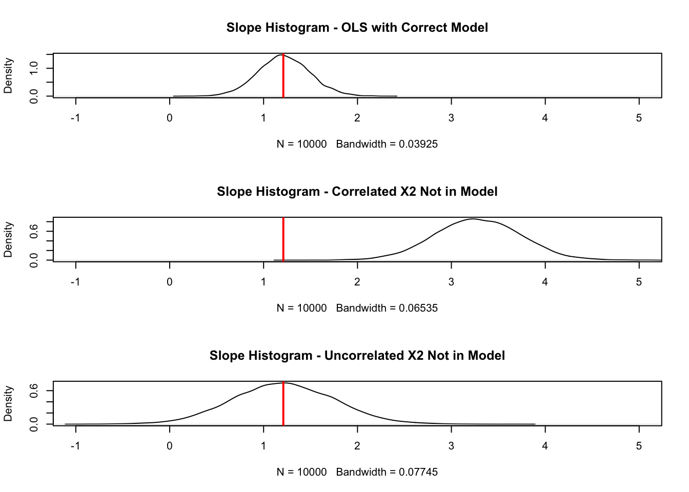
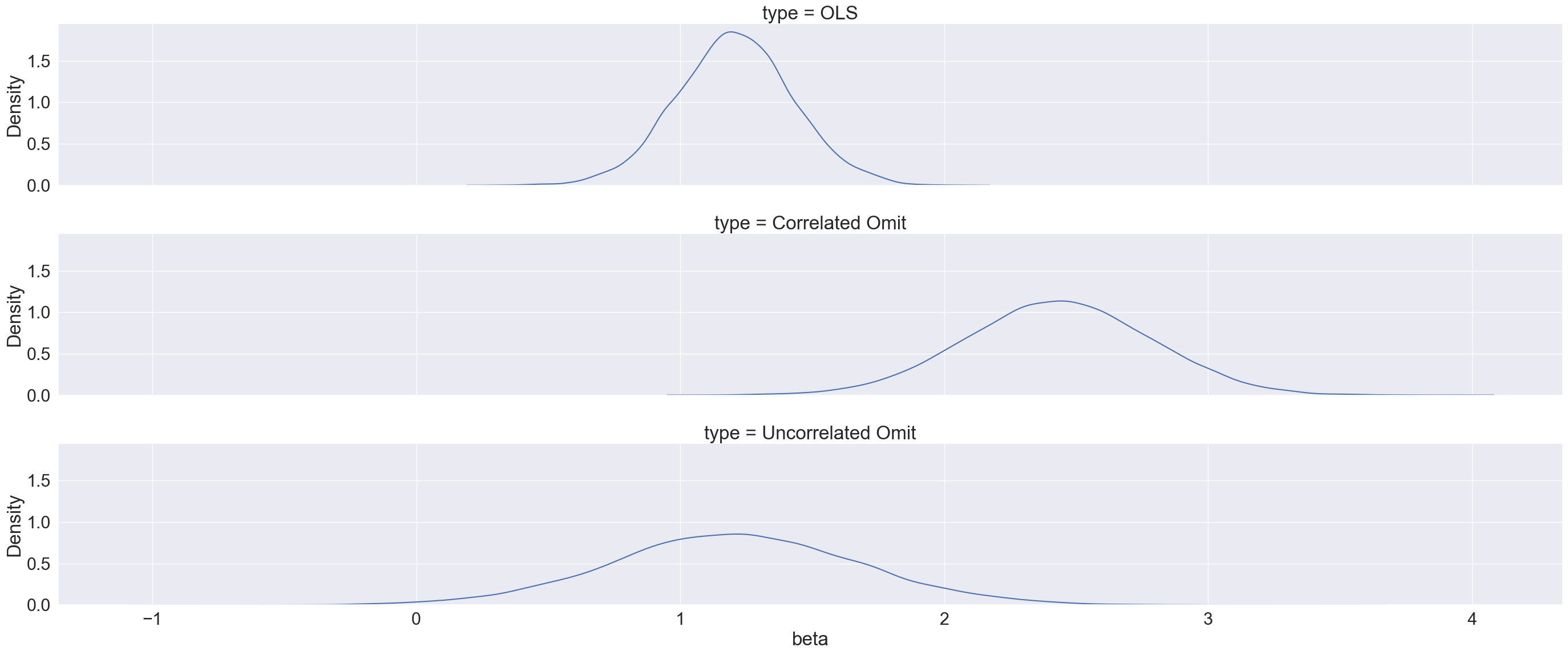
# Running regressions across every column. #all_results_c <-lapply(1:simulation.size, function(x) lm(Y.c[,x] ~ X1.c[,x]))all_results_uc <-lapply(1:simulation.size, function(x) lm(Y.uc[,x] ~ X1.c[,x]))all_results_ols <-lapply(1:simulation.size, function(x) lm(Y.c[,x] ~ X1.c[,x] + X2.c[,x]))# Gathering and plotting the distribution of the coefficients. #betas_c <-sapply(all_results_c, coef)betas_uc <-sapply(all_results_uc, coef)betas_ols <-sapply(all_results_ols, coef)par(mfrow=c(3,1))plot(density(betas_ols[2,]), xlim =c(-1,5), main ="Slope Histogram - OLS with Correct Model")abline(v =1.21, col="red", lwd=2)plot(density(betas_c[2,]), xlim =c(-1,5), main ="Slope Histogram - Correlated X2 Not in Model")abline(v =1.21, col="red", lwd=2)plot(density(betas_uc[2,]), xlim =c(-1,5), main ="Slope Histogram - Uncorrelated X2 Not in Model")abline(v =1.21, col="red", lwd=2)
Code
par(mfrow=c(1,1))
From the plots above we can see the impact of leaving out important variables that should be in our model. If our model leaves out a predictor variable that is correlated with another predictor variable, the coefficient of the predictor variable in the model is biased. Here we can see, the vertical lines showing the true value of the coefficient. When the omitted variable is correlated, our distribution of the coefficient of \(X_1\) is not centered around its true value. Even if the omitted variable isn’t correlated, we can see that the standard error (the spread) of the distribution of the coefficient for the variable \(X_1\) is still wider than it would be under the circumstance where we specified the model correctly.
Another thing we can check is how many times we incorrectly, fail to reject our null hypothesis that \(X_1\) isn’t a significant variable in our model. We know it is an important variable since we created the model. However, let’s look at the p-values for the coefficient on \(X_1\) for each of the simulations. We just use the sapply function to apply the summary function and extract the coefficients element from each linear regression. Then we just sum up how many times our p-value was above 0.05. This should NOT be the case too often since we know \(X_1\) should be in our model.
As you can see, in the correctly specified model, we incorrectly say \(X_1\) is not statistically significant only 1.17% of the time. However, when we left out our \(X_2\) variable and it wasn’t correlated, we make this mistake 41.24% of the time.
This simulation is a little more drawn out. First, we set the parameters of interest - sample size, simulation size, coefficients for the regression model, and the correlation between the X’s. Next, we calculate the Cholesky decomposition of our correlation matrix to help with correlating of data. From there we simulate three variables, \(X_1\), \(X_2\), and \(X_{2u}\). The first \(X_2\) we will correlate with \(X_1\), but we will leave \(X_{2u}\) uncorrelated with \(X_1\). Lastly, we correlate \(X_1\) and \(X_2\) as described in the above sections on correlated variables.
Now we need to create our models. In other words, we need to simulate our target variables under the conditions described above. We have two models to simulate. The first is Y_c where we have \(Y\) as a function of \(X_1\), \(X_2\), and our error, \(\varepsilon\), simulated from a normal distribution using random.normal. The second is Y_uc where we have \(Y\) as a function of \(X_1\), \(X_{2u}\), and our error, \(\varepsilon\), simulated from a normal distribution using random.normal.
Next, we just create columns for each simulation of our variables in datasets to loop across using the reshape function.
Now we get to run the regressions. We use a for loop to apply the ols function (for building linear regressions) from statsmodels.formula.api across all three types of models. The betas_c object has the linear regressions leaving out a correlated \(X_2\). The betas_uc object has the linear regressions leaving out a uncorrelated \(X_{2u}\). The betas_ols object has the correct linear regressions leaving out no variables. From there, we use the params function across each of our linear regressions to get the coefficients from \(X_1\) from each of the models.
From the plots above we can see the impact of leaving out important variables that should be in our model. If our model leaves out a predictor variable that is correlated with another predictor variable, the coefficient of the predictor variable in the model is biased. Here we can see, the vertical lines showing the true value of the coefficient. When the omitted variable is correlated, our distribution of the coefficient of \(X_1\) is not centered around its true value of 1.21. Even if the omitted variable isn’t correlated, we can see that the standard error (the spread) of the distribution of the coefficient for the variable \(X_1\) is still wider than it would be under the circumstance where we specified the model correctly.
This simulation is a little more drawn out. First, we set the parameters of interest - sample size, simulation size, coefficients for the regression model, and the correlation between the X’s using MACRO variables. Next, we build in the correlation structure between \(X_2\) and \(X_{2u}\) using the same approach as described in the correlation section above using DATA steps and PROC MODEL.
Code
%let Sample_Size =50;%let Simulation_Size =10000;%let Beta0 =-13;%let Beta1 =1.21;%let Beta2 =3.45;%let Correlation_Coef =0.6;/* Creating correlation matrices */data Corr_Matrix; do i =1 to &Simulation_Size; _type_ ="corr"; _name_ ="X_1"; X_1 =1.0; X_2 =&Correlation_Coef; output; _name_ ="X_2"; X_1 =&Correlation_Coef; X_2 =1.0; output; end;run;/* Creating initial values as place holders */data Naive; do i =1 to &Simulation_Size; X_1 =0; X_2 =0; output; end;run;/* Generate the correlated X_1 and X_2 */proc model noprint;/* Distributiuon of X_1 */ X_1 =0; errormodel X_1 ~Normal(1); /*Distribution of X_2*/ X_2 =0; errormodel X_2 ~Normal(1); /* Generate the data and store them in the dataset work.Correlated_X */ solve X_1 X_2 / random =&Sample_Size sdata = Corr_Matrix data = Naive out =Correlated_X(keep = X_1 X_2 i _rep_); by i; run;quit;data Correlated_X; set Correlated_X; by i;if first.i then delete; rename i = sim; rename _rep_ = obs;run;
Now we need to create our models. First, we will simulate our errors from the model, \(\varepsilon\) and our uncorrelated \(X_{2u}\) variable. Then we can merge all of our simulated data together in a DATA step with the MERGE statement. With this new combined dataset we have columns of all of our simulated variables across many simulated rows. All we then need to do is combine the columns into our target variables \(Y\) and \(Y_u\) for the model with correlated and uncorrelated inputs respectively.
Code
/* Generate Linear Regression Model Data */data simulation;do sim =1 to &Simulation_Size; do obs =1 to &Sample_Size; call streaminit(112358); err =sqrt(2.25)*rand('normal'); X_2u =sqrt(1)*rand('normal'); output; end;end;run;data all_data; merge simulation Correlated_X; by sim obs; Y =&Beta0 +&Beta1*X_1 +&Beta2*X_2 + err; Yu =&Beta0 +&Beta1*X_1 +&Beta2*X_2u + err;run;
Now we get to run the regressions. We use PROC REG to build all of our models by the variable sim using the BYstatement so we get results for each simulation’s rows. We store the output from all these regressions into a dataset called all_results using the OUTEST = option. We are complete with the simulation. Next we just clean up the results with some DATA step manipulation for labeling as well as a PROC SORT to make the visuals displayed in PROC SGPANEL nicer to see. The options in the plotting procedure aren’t covered in detail here as that is not the focus.
Code
/* Run all regressions and store the output */proc reg data = all_data outest = all_results tableout noprint; OLSC: model Y = X_1 X_2; Corr: model Y = X_1; UnCorr: model Yu = X_1; by sim;run;/* Give meaningful values to the _model_ variable */data all_results; set all_results; label _model_="Model";ifupcase(_model_) eq "Corr" then _model_="Omit Correl. X";elseifupcase(_model_) eq "UnCorr" then _model_="Omit Uncorrel. X"; elseifupcase(_model_) eq "OLSC" then _model_="Correct Model";run;/* Normal plots and univariate statistics for each variable/model */proc sort data=all_results; by _model_;run;/* Create a panel of plots, by model, to contrast normal vs. empirical distr. AKA Make things look pretty... *//* Also add a reference line that highlights the true parameter value */proc sgpanel data =all_results(where=(_type_ eq 'PARMS')); panelby _model_ / layout=ROWLATTICE uniscale=column columns=1 onepanel; density X_1 / type=kernel; refline &Beta1 / axis=x label="&Beta1" labelattrs=(weight=bold);run;
From the plots above we can see the impact of leaving out important variables that should be in our model. If our model leaves out a predictor variable that is correlated with another predictor variable, the coefficient of the predictor variable in the model is biased. Here we can see, the vertical lines showing the true value of the coefficient. When the omitted variable is correlated, our distribution of the coefficient of \(X_1\) is not centered around its true value. Even if the omitted variable isn’t correlated, we can see that the standard error (the spread) of the distribution of the coefficient for the variable \(X_1\) is still wider than it would be under the circumstance where we specified the model correctly.
Omitting important variables is a problem. If those variables are correlated with other inputs that are in the model, then our inputs in the model have biased estimations. However, even if they are not correlated and therefore unbiased, we make many more mistakes about our model input’s significance in the model.
Source Code
---title: "Theory Assessment"format: html: code-fold: show code-tools: trueeditor: visual---```{r}#| include: falselibrary(reticulate)use_condaenv("r-main")```# Closed Form SolutionsIn mathematics and statistics, there are popular theories involving distributions of known values. The Central Limit Theorem is one of them. We don't need complicated mathematics for us to approximate distributional assumptions when we use simulations. This is especially helpful when finding a **closed form solution** is very difficult, if not impossible. A closed form solution to a mathematical/statistical distribution problem means that you can mathematically calculate the distribution through equations. Real world data can be very complicated and may change based on different inputs which each have their own unique distribution. Simulation can reveal an approximation of these output distributions.The next two sections work through some examples of this.# Central Limit TheoremAssume you do not know the Central Limit Theorem, but want to study and understand the sampling distribution of sample means. You take samples of size 10, 50, and 100 from the following three population distributions and calculate the sample means repeatedly:1. Normal distribution2. Uniform distribution3. Exponential distributionLet's use our software to simulate the sampling distributions of sample means across each of the above distributions and sample sizes!::: {.panel-tabset .nav-pills}## RThis simulation can easily be done in R without the use of loops. First, we set the sample size and simulation size of the simulation. Next, we just randomly sample from each of the above distributions using the `rnorm`, `runif`, and `rexp` functions. In each of these functions we sample as many observations we would need across all simulations which is the product of the sample size with the simulation size. We then use the `matrix` function to take the draws from the random sampling functions and allocate the observations across rows and columns of a matrix. Specifically, we will use the rows as simulations, and columns as samples. Lastly, we just use the `apply` function for each matrix and apply the `mean` function to each row (or simulation). From there we can plot the distributions of the sample means.```{r}#| message: false#| error: false#| warning: falsesample.size <-50simulation.size <-10000X1 <-matrix(data=rnorm(n=(sample.size*simulation.size), mean=2, sd=5), nrow=simulation.size, ncol=sample.size, byrow=TRUE)X2 <-matrix(data=runif(n=(sample.size*simulation.size), min=5, max=105), nrow=simulation.size, ncol=sample.size, byrow=TRUE)X3 <-matrix(data=(rexp(n=(sample.size*simulation.size)) +3), nrow=simulation.size, ncol=sample.size, byrow=TRUE)Mean.X1 <-apply(X1,1,mean)Mean.X2 <-apply(X2,1,mean)Mean.X3 <-apply(X3,1,mean)hist(Mean.X1, breaks=50, main='Sample Distribution of Means for Normal Distribution', xlab='Sample Means')hist(Mean.X2, breaks=50, main='Sample Distribution of Means for Uniform Distribution', xlab='Sample Means')hist(Mean.X3, breaks=50, main='Sample Distribution of Means for Exponential Distribution', xlab='Sample Means')```The example above shows sampling distributions for the mean when the sample size is 50. Easily changing that piece of the code will allow the user to see these sampling distributions at different sample sizes.As you can see above, the sampling distribution for the sample means is approximately normally distributed, regardless of the population distribution, as long as the sample size is big enough.## PythonThis simulation can easily be done in Python without the use of loops. First, we set the sample size and simulation size of the simulation. Next, we just randomly sample from each of the above distributions using the `random.normal`, `random.uniform`, and `random.exponential` functions from `numpy`. In each of these functions we sample as many observations we would need across all simulations which is the product of the sample size with the simulation size. We then use the `reshape` function on these arrays to take the draws from the random sampling functions and allocate the observations across rows and columns of an array. Specifically, we will use the rows as simulations, and columns as samples. Lastly, we just use the `mean` function for each array and apply the `axis = 1` option to each row (or simulation). From there we can plot the distributions of the sample means.```{python}#| message: false#| error: false#| warning: falseimport numpy as npsample_size =50simulation_size =10000X1 = np.random.normal(loc =0.04, scale =0.07, size = sample_size*simulation_size).reshape(simulation_size, sample_size)X2 = np.random.uniform(low =5, high =105, size = sample_size*simulation_size).reshape(simulation_size, sample_size)X3 = np.random.exponential(scale =0.333, size = sample_size*simulation_size).reshape(simulation_size, sample_size)Mean_X1 = X1.mean(axis =1)Mean_X2 = X2.mean(axis =1)Mean_X3 = X3.mean(axis =1)``````{python}#| message: false#| error: false#| warning: falseimport seaborn as snsimport matplotlib.pyplot as pltax = sns.histplot(data = Mean_X1)ax.set_title('Sample Distribution of Means for Normal Distribution')ax.set_xlabel("Sample Means")``````{python}#| message: false#| error: false#| warning: falseax = sns.histplot(data = Mean_X2)ax.set_title('Sample Distribution of Means for Uniform Distribution')ax.set_xlabel("Sample Means")``````{python}#| message: false#| error: false#| warning: falseax = sns.histplot(data = Mean_X3)ax.set_title('Sample Distribution of Means for Exponential Distribution')ax.set_xlabel("Sample Means")```The example above shows sampling distributions for the mean when the sample size is 50. Easily changing that piece of the code will allow the user to see these sampling distributions at different sample sizes.As you can see above, the sampling distribution for the sample means is approximately normally distributed, regardless of the population distribution, as long as the sample size is big enough.## SASThis simulation can easily be done in SAS with a couple of loops in a `DATA` step. First, we set the sample size and simulation size of the simulation with MACRO variables using the `%` symbol. Next, we open two `DO` loops to loop over the simulation and sample size. Then we just randomly sample from each of the above distributions using the `RAND` function with the `Normal`, `Uniform`, and `Exponential` options. We then use the `OUTPUT` statement to make sure that the results from each iteration in the loop are stored as a separate row in the dataset. Lastly, we just use the `PROC MEANS` procedure to calculate the means across each variable (using the `VAR` statement) for each simulation (using the `BY` statement). We use the `OUTPUT` statement and `OUT` option to store the resulting means into separate datasets as different columns - one column for each simulation. From there we can plot the distributions of the sample means using three separate `SGPLOT` procedure calls.```{r}#| eval: false%let Sample_Size =50;%let Simulation_Size =10000;data CLT; do sim =1 to &Simulation_Size; do obs =1 to &Sample_Size; call streaminit(12345); X1 =RAND('Normal', 2, 5); X2 =5+100*RAND('Uniform'); X3 =3+RAND('Exponential'); output; end; end;run;proc means data=CLT noprint mean; var X1 X2 X3; by sim; output out=Means mean(X1 X2 X3)=Mean_X1 Mean_X2 Mean_X3;run;proc sgplot data=Means; title 'Sampling Distribution of Means'; title2 'Normal Distribution'; histogram Mean_X1; keylegend / location=inside position=topright;run;proc sgplot data=Means; title 'Sampling Distribution of Means'; title2 'Uniform Distribution'; histogram Mean_X2; keylegend / location=inside position=topright;run;proc sgplot data=Means; title 'Sampling Distribution of Means'; title2 'Exponential Distribution'; histogram Mean_X3; keylegend / location=inside position=topright;run;```{fig-align="center" width="7in"}{fig-align="center" width="7in"}{fig-align="center" width="7in"}The example above shows sampling distributions for the mean when the sample size is 50. Easily changing that piece of the code will allow the user to see these sampling distributions at different sample sizes.As you can see above, the sampling distribution for the sample means is approximately normally distributed, regardless of the population distribution, as long as the sample size is big enough.:::# Omitted Variable BiasWhat if you leave an important variable out of a linear regression that should have been in the model? From statistical theory it would change the bias of the coefficients in the model as well as the variability of the coefficients, depending on if the variable left out was correlated with another variable in the model. Simulation can help us show this as well as determine how bad these problems could get under different circumstances.Let's simulate the following regression model:$$Y = -13 + 1.21X_1 + 3.45X_2 + \varepsilon$$Assume that the errors, $\varepsilon$ , in the model above are normally distributed with a mean of 0 and standard deviation of 1.5. Also assume that the predictors $X_1$ and $X_2$ are normally distributed with mean of 0 and standard deviation of 1. Build 10,000 linear regressions (each of sample size 50) and record the coefficients from the regression models for each of these simulations:1. Model with both $X_1$ and $X_2$ in the model2. Model with only $X_1$ in the model and $X_2$ with the correlation between the two as 0.63. Model with only $X_1$ in the model and $X_2$ with the correlation between the two as 0Let's see the simulations in our software!::: {.panel-tabset .nav-pills}## RThis simulation is a little more drawn out. First, we set the parameters of interest - sample size, simulation size, coefficients for the regression model, and the correlation between the X's. Next, we calculate the Cholesky decomposition of our correlation matrix to help with correlating of data. From there we simulate three variables, $X_1$, $X_2$, and $X_{2u}$. The first $X_2$ we will correlate with $X_1$, but we will leave $X_{2u}$ uncorrelated with $X_1$. Lastly, we correlate $X_1$ and $X_2$ as described in the above sections on correlated variables.```{r}#| message: false#| error: false#| warning: false#| echo: falsestandardize <-function(x){ x.std = (x -mean(x))/sd(x)return(x.std)}destandardize <-function(x.std, x){ x.old = (x.std *sd(x)) +mean(x)return(x.old)}``````{r}#| message: false#| error: false#| warning: falsesample.size <-50simulation.size <-10000beta0 <--13beta1 <-1.21beta2 <-3.45correlation_coef <-0.6R <-matrix(data=cbind(1,correlation_coef, correlation_coef, 1), nrow=2)U <-t(chol(R))set.seed(112358)X1 <-rnorm(sample.size*simulation.size, mean =0, sd =1)X2 <-rnorm(sample.size*simulation.size, mean =0, sd =1)X2u <-rnorm(sample.size*simulation.size, mean =0, sd =1)Both <-cbind(X1, X2)X1X2 <- U %*%t(Both)X1X2 <-t(X1X2)```Now we need to create our models. In other words, we need to simulate our target variables under the conditions described above. We have two models to simulate. The first is *Y.c* where we have $Y$ as a function of $X_1$, $X_2$, and our error, $\varepsilon$, simulated from a normal distribution using `rnorm`. The second is *Y.uc* where we have $Y$ as a function of $X_1$, $X_{2u}$, and our error, $\varepsilon$, simulated from a normal distribution using `rnorm`.Next, we just create columns for each simulation of our variables in datasets to loop across.```{r}#| message: false#| error: false#| warning: false# Time to create the two target variables - one with correlated X's, one without. #all_data <-data.frame(X1X2)all_data$Y.c <- beta0 + beta1*all_data$X1 + beta2*all_data$X2 +rnorm(sample.size*simulation.size, mean =0, sd =1.5)all_data$Y.u <- beta0 + beta1*all_data$X1 + beta2*X2u +rnorm(sample.size*simulation.size, mean =0, sd =1.5)# Getting all the data in separate columns to loop across. #X1.c <-data.frame(matrix(all_data$X1, ncol = simulation.size))X2.c <-data.frame(matrix(all_data$X2, ncol = simulation.size))X2.uc <-data.frame(matrix(X2u, ncol = simulation.size))Y.c <-data.frame(matrix(all_data$Y.c, ncol = simulation.size))Y.uc <-data.frame(matrix(all_data$Y.u, ncol = simulation.size))```Now we get to run the regressions. We use `lapply` to apply the `lm` function (for building linear regressions) across all three types of models. The *all_results_c* object has the linear regressions leaving out a correlated $X_2$. The *all_results_uc* object has the linear regressions leaving out a uncorrelated $X_{2u}$. The *all_results_ols* object has the correct linear regressions leaving out no variables. From there, we use the `sapply` function to apply the `coef` function across each of our linear regressions to get the coefficients from the models. Lastly, we just plot the densities of the coefficients from each of the three scenarios using the `density` function.```{r}#| message: false#| error: false#| warning: false# Running regressions across every column. #all_results_c <-lapply(1:simulation.size, function(x) lm(Y.c[,x] ~ X1.c[,x]))all_results_uc <-lapply(1:simulation.size, function(x) lm(Y.uc[,x] ~ X1.c[,x]))all_results_ols <-lapply(1:simulation.size, function(x) lm(Y.c[,x] ~ X1.c[,x] + X2.c[,x]))# Gathering and plotting the distribution of the coefficients. #betas_c <-sapply(all_results_c, coef)betas_uc <-sapply(all_results_uc, coef)betas_ols <-sapply(all_results_ols, coef)par(mfrow=c(3,1))plot(density(betas_ols[2,]), xlim =c(-1,5), main ="Slope Histogram - OLS with Correct Model")abline(v =1.21, col="red", lwd=2)plot(density(betas_c[2,]), xlim =c(-1,5), main ="Slope Histogram - Correlated X2 Not in Model")abline(v =1.21, col="red", lwd=2)plot(density(betas_uc[2,]), xlim =c(-1,5), main ="Slope Histogram - Uncorrelated X2 Not in Model")abline(v =1.21, col="red", lwd=2)par(mfrow=c(1,1))```From the plots above we can see the impact of leaving out important variables that should be in our model. If our model leaves out a predictor variable that is correlated with another predictor variable, the coefficient of the predictor variable **in** the model is biased. Here we can see, the vertical lines showing the true value of the coefficient. When the omitted variable is correlated, our distribution of the coefficient of $X_1$ is not centered around its true value. Even if the omitted variable isn't correlated, we can see that the standard error (the spread) of the distribution of the coefficient for the variable $X_1$ is still wider than it would be under the circumstance where we specified the model correctly.Another thing we can check is how many times we incorrectly, fail to reject our null hypothesis that $X_1$ isn't a significant variable in our model. We know it is an important variable since we created the model. However, let's look at the p-values for the coefficient on $X_1$ for each of the simulations. We just use the `sapply` function to apply the `summary` function and extract the `coefficients` element from each linear regression. Then we just sum up how many times our p-value was above 0.05. This should **NOT** be the case too often since we know $X_1$ should be in our model.```{r}#| message: false#| error: false#| warning: falsepval_c <-sapply(all_results_c, function(x) summary(x)$coefficients[2,4])pval_uc <-sapply(all_results_uc, function(x) summary(x)$coefficients[2,4])pval_ols <-sapply(all_results_ols, function(x) summary(x)$coefficients[2,4])(sum(pval_ols >0.05)/10000)*100(sum(pval_c >0.05)/10000)*100(sum(pval_uc >0.05)/10000)*100```As you can see, in the correctly specified model, we incorrectly say $X_1$ is not statistically significant only 1.17% of the time. However, when we left out our $X_2$ variable and it wasn't correlated, we make this mistake 41.24% of the time.## PythonThis simulation is a little more drawn out. First, we set the parameters of interest - sample size, simulation size, coefficients for the regression model, and the correlation between the X's. Next, we calculate the Cholesky decomposition of our correlation matrix to help with correlating of data. From there we simulate three variables, $X_1$, $X_2$, and $X_{2u}$. The first $X_2$ we will correlate with $X_1$, but we will leave $X_{2u}$ uncorrelated with $X_1$. Lastly, we correlate $X_1$ and $X_2$ as described in the above sections on correlated variables.```{python}#| message: false#| error: false#| warning: falseimport numpy as npimport scipy as spsample_size =50simulation_size =10000beta0 =-13beta1 =1.21beta2 =3.45correlation_coef =0.6R = np.array([[1, correlation_coef], [correlation_coef, 1]])U = sp.linalg.cholesky(R, lower =False)X1 = np.random.normal(loc =0, scale =1, size = sample_size*simulation_size)X2 = np.random.normal(loc =0, scale =1, size = sample_size*simulation_size)X2u = np.random.normal(loc =0, scale =1, size = sample_size*simulation_size)Both = np.array([X1, X2])X1X2 = U @ BothX1X2 = np.transpose(X1X2)```Now we need to create our models. In other words, we need to simulate our target variables under the conditions described above. We have two models to simulate. The first is *Y_c* where we have $Y$ as a function of $X_1$, $X_2$, and our error, $\varepsilon$, simulated from a normal distribution using `random.normal`. The second is *Y_uc* where we have $Y$ as a function of $X_1$, $X_{2u}$, and our error, $\varepsilon$, simulated from a normal distribution using `random.normal`.Next, we just create columns for each simulation of our variables in datasets to loop across using the `reshape` function.```{python}#| message: false#| error: false#| warning: falseimport pandas as pdall_data = pd.DataFrame(X1X2)all_data.columns = ['X1', 'X2']all_data['Y_c'] = beta0 + beta1*all_data['X1'] + beta2*all_data['X2'] + np.random.normal(loc =0, scale =1.5, size = sample_size*simulation_size)all_data['Y_u'] = beta0 + beta1*all_data['X1'] + beta2*X2u + np.random.normal(loc =0, scale =1.5, size = sample_size*simulation_size)X1_c = pd.DataFrame(np.array([all_data['X1']]).reshape(simulation_size, sample_size))X2_c = pd.DataFrame(np.array([all_data['X2']]).reshape(simulation_size, sample_size))X2_uc = pd.DataFrame(np.array([X2u]).reshape(simulation_size, sample_size))Y_c = pd.DataFrame(np.array([all_data['Y_c']]).reshape(simulation_size, sample_size))Y_uc = pd.DataFrame(np.array([all_data['Y_u']]).reshape(simulation_size, sample_size))```Now we get to run the regressions. We use a `for` loop to apply the `ols` function (for building linear regressions) from `statsmodels.formula.api` across all three types of models. The *betas_c* object has the linear regressions leaving out a correlated $X_2$. The *betas_uc* object has the linear regressions leaving out a uncorrelated $X_{2u}$. The *betas_ols* object has the correct linear regressions leaving out no variables. From there, we use the `params` function across each of our linear regressions to get the coefficients from $X_1$ from each of the models.```{python}#| message: false#| error: false#| warning: falseimport statsmodels.formula.api as smfbetas_c = []for i inrange(10000): df_array = np.array([Y_c.iloc[i,], X1_c.iloc[i,]]) df = pd.DataFrame(np.transpose(df_array)) df.columns = ['Y_c', 'X1_c'] model = smf.ols('Y_c ~ X1_c', data = df).fit() beta = model.params['X1_c'] betas_c.append(beta)betas_c = pd.DataFrame(betas_c)betas_c.columns = ['beta']betas_uc = []for i inrange(10000): df_array = np.array([Y_uc.iloc[i,], X1_c.iloc[i,]]) df = pd.DataFrame(np.transpose(df_array)) df.columns = ['Y_uc', 'X1_c'] model = smf.ols('Y_uc ~ X1_c', data = df).fit() beta = model.params['X1_c'] betas_uc.append(beta)betas_uc = pd.DataFrame(betas_uc)betas_uc.columns = ['beta']betas_ols = []for i inrange(10000): df_array = np.array([Y_c.iloc[i,], X1_c.iloc[i,], X2_c.iloc[i,]]) df = pd.DataFrame(np.transpose(df_array)) df.columns = ['Y_c', 'X1_c', 'X2_c'] model = smf.ols('Y_c ~ X1_c + X2_c', data = df).fit() beta = model.params['X1_c'] betas_ols.append(beta)betas_ols = pd.DataFrame(betas_ols)betas_ols.columns = ['beta']```Now we just plot the densities of the beta distributions from each of the regression simulations above using the `kdeplot` from `seaborn`.```{python}#| message: false#| error: false#| warning: falseimport seaborn as snsbetas_ols['type'] ='OLS'betas_c['type'] ='Correlated Omit'betas_uc['type'] ='Uncorrelated Omit'betas_all = pd.concat([betas_ols, betas_c, betas_uc])sns.set(font_scale =2)grid = sns.FacetGrid(betas_all, row ='type', height =4, aspect =7)grid.map(sns.kdeplot, 'beta')```From the plots above we can see the impact of leaving out important variables that should be in our model. If our model leaves out a predictor variable that is correlated with another predictor variable, the coefficient of the predictor variable **in** the model is biased. Here we can see, the vertical lines showing the true value of the coefficient. When the omitted variable is correlated, our distribution of the coefficient of $X_1$ is not centered around its true value of 1.21. Even if the omitted variable isn't correlated, we can see that the standard error (the spread) of the distribution of the coefficient for the variable $X_1$ is still wider than it would be under the circumstance where we specified the model correctly.## SASThis simulation is a little more drawn out. First, we set the parameters of interest - sample size, simulation size, coefficients for the regression model, and the correlation between the X's using MACRO variables. Next, we build in the correlation structure between $X_2$ and $X_{2u}$ using the same approach as described in the correlation section above using `DATA` steps and `PROC MODEL`.```{r}#| eval: false%let Sample_Size =50;%let Simulation_Size =10000;%let Beta0 =-13;%let Beta1 =1.21;%let Beta2 =3.45;%let Correlation_Coef =0.6;/* Creating correlation matrices */data Corr_Matrix; do i =1 to &Simulation_Size; _type_ ="corr"; _name_ ="X_1"; X_1 =1.0; X_2 =&Correlation_Coef; output; _name_ ="X_2"; X_1 =&Correlation_Coef; X_2 =1.0; output; end;run;/* Creating initial values as place holders */data Naive; do i =1 to &Simulation_Size; X_1 =0; X_2 =0; output; end;run;/* Generate the correlated X_1 and X_2 */proc model noprint;/* Distributiuon of X_1 */ X_1 =0; errormodel X_1 ~Normal(1); /*Distribution of X_2*/ X_2 =0; errormodel X_2 ~Normal(1); /* Generate the data and store them in the dataset work.Correlated_X */ solve X_1 X_2 / random =&Sample_Size sdata = Corr_Matrix data = Naive out =Correlated_X(keep = X_1 X_2 i _rep_); by i; run;quit;data Correlated_X; set Correlated_X; by i;if first.i then delete; rename i = sim; rename _rep_ = obs;run;```Now we need to create our models. First, we will simulate our errors from the model, $\varepsilon$ and our uncorrelated $X_{2u}$ variable. Then we can merge all of our simulated data together in a `DATA` step with the `MERGE` statement. With this new combined dataset we have columns of all of our simulated variables across many simulated rows. All we then need to do is combine the columns into our target variables $Y$ and $Y_u$ for the model with correlated and uncorrelated inputs respectively.```{r}#| eval: false/* Generate Linear Regression Model Data */data simulation;do sim =1 to &Simulation_Size; do obs =1 to &Sample_Size; call streaminit(112358); err =sqrt(2.25)*rand('normal'); X_2u =sqrt(1)*rand('normal'); output; end;end;run;data all_data; merge simulation Correlated_X; by sim obs; Y =&Beta0 +&Beta1*X_1 +&Beta2*X_2 + err; Yu =&Beta0 +&Beta1*X_1 +&Beta2*X_2u + err;run;```Now we get to run the regressions. We use `PROC REG` to build all of our models by the variable *sim* using the `BY`statement so we get results for each simulation's rows. We store the output from all these regressions into a dataset called *all_results* using the `OUTEST =` option. We are complete with the simulation. Next we just clean up the results with some `DATA` step manipulation for labeling as well as a `PROC SORT` to make the visuals displayed in `PROC SGPANEL` nicer to see. The options in the plotting procedure aren't covered in detail here as that is not the focus.```{r}#| eval: false/* Run all regressions and store the output */proc reg data = all_data outest = all_results tableout noprint; OLSC: model Y = X_1 X_2; Corr: model Y = X_1; UnCorr: model Yu = X_1; by sim;run;/* Give meaningful values to the _model_ variable */data all_results; set all_results; label _model_="Model";ifupcase(_model_) eq "Corr" then _model_="Omit Correl. X";elseifupcase(_model_) eq "UnCorr" then _model_="Omit Uncorrel. X"; elseifupcase(_model_) eq "OLSC" then _model_="Correct Model";run;/* Normal plots and univariate statistics for each variable/model */proc sort data=all_results; by _model_;run;/* Create a panel of plots, by model, to contrast normal vs. empirical distr. AKA Make things look pretty... *//* Also add a reference line that highlights the true parameter value */proc sgpanel data =all_results(where=(_type_ eq 'PARMS')); panelby _model_ / layout=ROWLATTICE uniscale=column columns=1 onepanel; density X_1 / type=kernel; refline &Beta1 / axis=x label="&Beta1" labelattrs=(weight=bold);run;```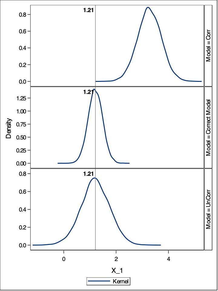{fig-align="center" width="7in"}From the plots above we can see the impact of leaving out important variables that should be in our model. If our model leaves out a predictor variable that is correlated with another predictor variable, the coefficient of the predictor variable in the model is biased. Here we can see, the vertical lines showing the true value of the coefficient. When the omitted variable is correlated, our distribution of the coefficient of $X_1$ is not centered around its true value. Even if the omitted variable isn't correlated, we can see that the standard error (the spread) of the distribution of the coefficient for the variable $X_1$ is still wider than it would be under the circumstance where we specified the model correctly.:::Omitting important variables is a problem. If those variables are correlated with other inputs that are in the model, then our inputs in the model have biased estimations. However, even if they are not correlated and therefore unbiased, we make many more mistakes about our model input's significance in the model.