Simulation
Instructor: Dr. Aric LaBarr
Introduction
Most analysis assumes a rather unrealistic view of the real world - certainty. In a real world setting - especially the business world - the inputs and coefficients in a problem are rarely fixed quantities. One possible solution to this is sensitivity analysis (like reduced cost and shadow prices) in optimization. However, a very popular approach to handling this uncertainty and trying to evalutate the effects of uncertainty are simulations.
Simulations help us determine not only the full array of outcomes of a given decision, but the probabilities of these outcomes occurring. These are extremely useful in many fields. Simulations - like target shuffling - are used to evaluate how likely your model occurred due to random chance. The field of risk management tries to simulate rare outcomes and measure their impact. This code deck will only cover the concept of simulation in general as well as some basic examples. For a full introduction to risk management please see the Introduction to Risk Management code deck.
What is the general idea behind simulation analysis? A fixed (or constant) input to a deterministic model will lead to a fixed output. Instead, in a simulation analysis, each input of a model (or process) is assigned a range of possible values - the probability distribution of the inputs. We then analyze what happens to the decision from our model (or process) under all these possiblre scenarios. Simulation analysis describes not only the outcomes of the certain decisions, but also the probability distribution of those outcomes. This helps us determine the probability that each of these outcomes occurs. For example, assume a stock price is $100 today. Next, let’s assume that it follows a random walk (random up or down movement centered at 0) each day for the next 100 days. This random walk follows a Gaussian (normal) distribution with a mean of 0 and standard deviation of 1. Let’s simulate some potential paths for this stock and compare them to the actual path.
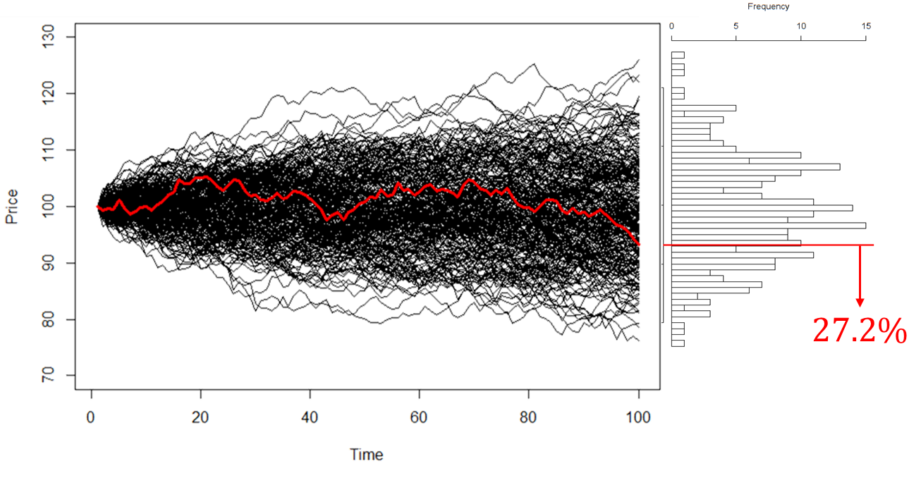
After the simulation is complete, the analysis turns to the probability distribution of the outcomes. We can calculate probabilities of outcomes or describe characteristics of this new distribution such as the mean, median, variance, skewness, percentiles, etc. From our example above we have a distrobution of possible prices that the stock can take after 100 days. In all those possible values, only 27.2% of them had a lower stock price.